Seasonal Unit Root Testing
An important element of time series data is seasonality or cyclicality. Typically, seasonality is treated as a stationary feature in most time series models. Nevertheless, non-stationarity, particularly of the unit-root kind, can be an important feature within the cyclical components themselves, and can give rise to similar inferential inaccuracies and concerns one often encounters with traditional unit root series. Accordingly, identifying the presence of unit roots at one or more seasonal frequencies is the subject of the battery of tests known as seasonal unit root tests.
EViews offers several seasonal unit root tests, including the classical Hylleberg, et al. (1990) test, the Smith and Taylor (1999) likelihood ratio test, the Canova and Hansen (1995) test, the Taylor (2003) robust stationarity test, and the Taylor (2005) variance ratio test.
The discussion to follow assumes familiarity with the theory of seasonal unit root tests.
Performing a Seasonal Unit Root Test in EViews
To begin, double click on a series name to open the series window. From there, select
To carry out a seasonal unit root test, there are three settings which must be specified.
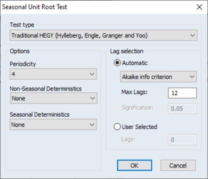
First, a test type should be chosen from the dropdown . Here, one of four tests can be selected.
• Traditional Hylleberg, Engle, Granger, and Yoo (HEGY) test
• HEGY Likelihood Ratio test
• Canova-Hansen test
• Variance ratio test
In the group, three options should be specified: , , and :
• Under one can select the seasonal frequency. EViews offers
as choices.
• Next, under the , one can select either , , or .
• Similarly, for , one can select , , , or . Note that some options are not available for all tests. For instance, the traditional HEGY test does not support spectral intercepts (and trends), and the Canova-Hansen test does not support non-seasonal trends.
Furthermore, the traditional HEGY and the HEGY Likelihood Ratio test allow for configuration of the procedures. In particular, one can select either automatic or user-specified lag selection. The default procedure is automatic selection using the AIC, but automatic selection supports:
• Akaike (AIC)
• Schwarz (SIC)
• Hannan-Quinn (HQ)
• t-Statistic
For the automatic selection methods, one must specify the maximum number of lags to consider (by default, 12), and, in the case of the t-statistic procedure, the significance level (by default, 0.05).
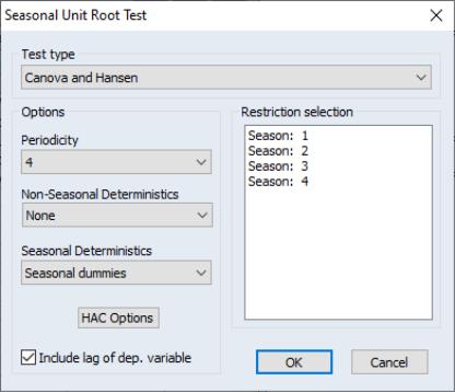
Note that additional options are displayed when carrying out the Canova-Hansen test:
• First, one can also configure long-run covariance estimation options by clicking on the button. Here, you may tweak the kernel, bandwidth, and pre-whitening settings.
• Further, note that the Canova-Hansen test also defaults to including a lag of the dependent variable as an additional exogenous regressor. This can be removed by deselecting the appropriate checkbox beneath the button.
• Specification of spectral frequencies to be tested can be selected in the checkbox. Note that when no frequencies are selected (default), all frequencies are tested.
Lastly, note that critical values for the traditional and likelihood-ratio HEGY tests have been computed by simulation, and in cases where relevant, linear interpolation is provided to adjust to actual sample sizes.
Examples
To illustrate the computation of seasonal root tests, we will use the famous airline passenger data from (“airpassengers.wf1”) which is a monthly dataset of total international airline passengers from 1949 to 1960.
We start with the traditional HEGY test using the default settings. Open the AIRPASSENGERS series and click on to display the dialog:
Click on to compute the tests at the default settings and display the results.
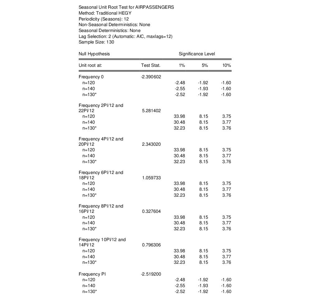
The top portion of the results, which describes the basics settings for the test and provides relevant test statistics for frequency

, frequency

, and the remaining 5 harmonic pair frequencies

for

. of the output is given below:
For each test statistic, critical values are given at the 1%, 5%, and 10% levels. In addition, since critical values are computed via simulation for sample sizes in intervals of 20, three sets of critical values are provided for each test. The interpolated value for the actual sample size, which in this case is

, and the closest lower and upper values for which simulations exist. In this case, the latter two are

and

:
The basic results are followed by results for joint tests of all seasonal frequencies and all frequencies, respectively:
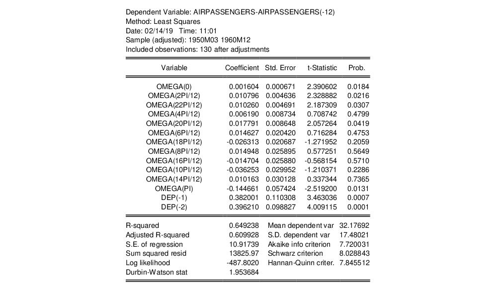
The bottom portion shows the HEGY test regression output:
Observe that in this example, the automatic lag selection has chosen 2 lags of the dependent variable to be used as additional regressors. These are captured as variables DEP(-1) and DEP(-2).
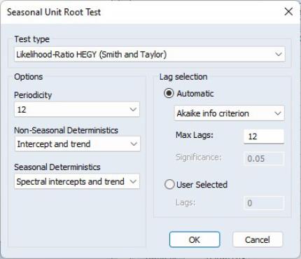
Next, we compute the HEGY likelihood ratio test, with a constant and trend, and spectral intercepts and trends:
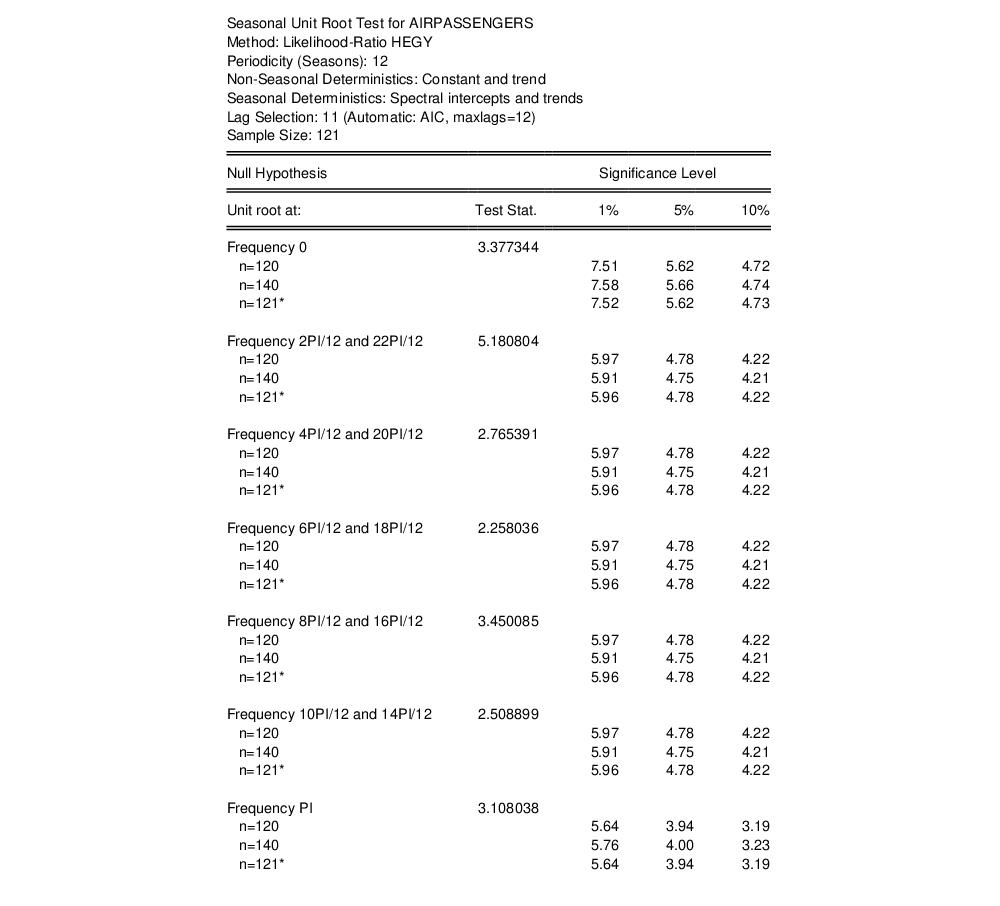
The top portion of output is:
The output is similar to that of the traditional HEGY test. The primary difference is that statistics are all computed as F-statistic and so all statistics are positive. Furthermore, since we have included spectral intercepts and trends, the latter variables are shown in the regression output in the second table. Not depicted here are the results for the joint tests, and the test regression equation.
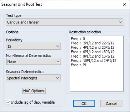
Next, consider the Canova-Hansen test performed on the same data. Here, we specify spectral intercepts and use defaults for everything else:
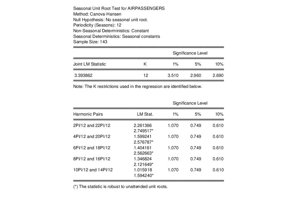
For the Canova-Hansen test, there are four sections of output.
The first section displays the joint test statistic, along with the total number of restrictions imposed, and the relevant critical values. In the second section, each of the harmonic pairs used in the joint test statistic is tested individually. Note here that each of the harmonic restrictions has two test statistics. The statistic without the asterisk is the usual CH test statistic. The asterisk marked statistic is robust to unattended unit roots.
The third section shows individual test statistics (in this case 12 of them), where the restrictions are tested on an individual basis. Note that the test statistics that are robust to unattended unit roots are reported here for frequencies

and

:
Finally, the last table consists of the test regression output:
Our final example computes the Taylor variance ratio test. We will again stick with the default settings:
In this case, the table provides test statistics for each of the frequencies

, frequency

, and the 5 harmonic pair frequencies

for

, along with the relevant critical values: