Estimating ARCH Models in EViews
To estimate an ARCH or GARCH model, open the equation specification dialog by selecting , by selecting . Select from the method dropdown menu at the bottom of the dialog. Alternately, typing the keyword arch in the command line both creates the object and sets the estimation method.
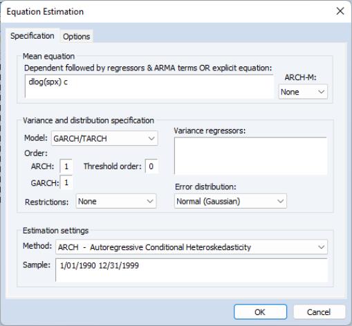
The dialog will change to show you the ARCH specification dialog. You will need to specify both the mean and the variance specifications, the error distribution and the estimation sample.
The Mean Equation
In the dependent variable edit box, you should enter the specification of the mean equation. You can enter the specification in list form by listing the dependent variable followed by the regressors. You should add the C to your specification if you wish to include a constant. If you have a more complex mean specification, you can enter your mean equation using an explicit expression.
If your specification includes an ARCH-M term, you should select the appropriate item of the dropdown menu in the upper right-hand side of the dialog. You may choose to include , , or the in the mean equation.
The Variance Equation
Your next step is to specify your variance equation.
Class of models
To estimate one of the standard GARCH models as described above, select the entry in the dropdown menu. The other entries (, , and C) correspond to more complicated variants of the GARCH specification. We discuss each of these models in
“Additional ARCH Models”.
In the section, you should choose the number of ARCH and GARCH terms. The default, which includes one ARCH and one GARCH term is by far the most popular specification.
If you wish to estimate an asymmetric model, you should enter the number of asymmetry terms in the r edit field. The default settings estimate a symmetric model with threshold order 0.
Variance regressors
In the edit box, you may optionally list variables you wish to include in the variance specification. Note that, with the exception of IGARCH models, EViews will always include a constant as a variance regressor so that you do not need to add C to this list.
The distinction between the permanent and transitory regressors is discussed in
“The Component GARCH (CGARCH) Model”.
Restrictions
If you choose the GARCH/TARCH model, you may restrict the parameters of the GARCH model in two ways. One option is to set the dropdown to IGARCH, which restricts the persistent parameters to sum up to one. Another is Variance Target, which restricts the constant term to a function of the GARCH parameters and the unconditional variance:
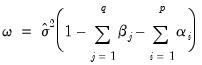 | (27.13) |
where

is the unconditional variance of the residuals.
The Error Distribution
To specify the form of the conditional distribution for your errors, you should select an entry from the dropdown menu.You may choose between the default the , the , the , or the . In the latter two cases, you will be prompted to enter a value for the fixed parameter. See
“Distributional Assumptions” for details on the supported distributions.
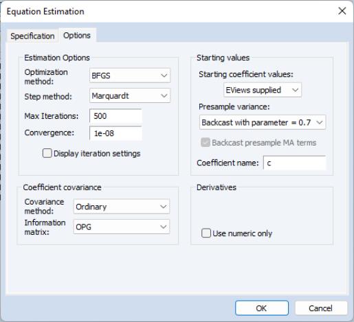
Estimation Options
EViews provides you with access to a number of optional estimation settings. Simply click on the Options tab and fill out the dialog as desired.
Backcasting
By default, both the innovations used in initializing MA estimation and the initial variance required for the GARCH terms are computed using backcasting methods. Details on the MA backcasting procedure are provided in
“Initializing MA Innovations”.
When computing backcast initial variances for GARCH, EViews first uses the coefficient values to compute the residuals of the mean equation, and then computes an exponential smoothing estimator of the initial values,
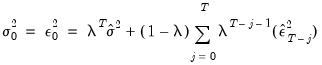 | (27.14) |
where

are the residuals from the mean equation,

is the unconditional variance estimate:
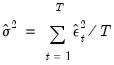 | (27.15) |
and the smoothing parameter

. However, you have the option to choose from a number of weights from 0.1 to 1, in increments of 0.1, by using the
Presample variance drop-down list. Notice that if the parameter is set to 1, then the initial value is simply the unconditional variance, e.g. backcasting is not calculated:
 | (27.16) |
Using the unconditional variance provides another common way to set the presample variance.
Our experience has been that GARCH models initialized using backcast exponential smoothing often outperform models initialized using the unconditional variance.
Heteroskedasticity Consistent Covariances
Click on the check box labeled Heteroskedasticity Consistent Covariance to compute the quasi-maximum likelihood (QML) covariances and standard errors using the methods described by Bollerslev and Wooldridge (1992). This option is only available if you choose the conditional normal as the error distribution.
You should use this option if you suspect that the residuals are not conditionally normally distributed. When the assumption of conditional normality does not hold, the ARCH parameter estimates will still be consistent, provided the mean and variance functions are correctly specified. The estimates of the covariance matrix will not be consistent unless this option is specified, resulting in incorrect standard errors.
Note that the parameter estimates will be unchanged if you select this option; only the estimated covariance matrix will be altered.
Derivative Methods
EViews uses both numeric and analytic derivatives in estimating ARCH models. Fully analytic derivatives are available for GARCH(p, q) models with simple mean specifications assuming normal or unrestricted t-distribution errors.
Analytic derivatives are not available for models with ARCH in mean specifications, complex variance equation specifications (e.g. threshold terms, exogenous variance regressors, or integrated or target variance restrictions), models with certain error assumptions (e.g. errors following the GED or fixed parameter t-distributions), and all non-GARCH(p, q) models (e.g. EGARCH, PARCH, component GARCH).
Some specifications offer analytic derivatives for a subset of coefficients. For example, simple GARCH models with non-constant regressors allow for analytic derivatives for the variance coefficients but use numeric derivatives for any non-constant regressor coefficients.
You may control the method used in computing numeric derivatives to favor speed (fewer function evaluations) or to favor accuracy (more function evaluations).
Iterative Estimation Control
The likelihood functions of ARCH models are not always well-behaved so that convergence may not be achieved with the default estimation settings. You can use the options dialog to select the iterative algorithm (Marquardt, BHHH/Gauss-Newton), change starting values, increase the maximum number of iterations, or adjust the convergence criterion.
Starting Values
As with other iterative procedures, starting coefficient values are required. EViews will supply its own starting values for ARCH procedures using OLS regression for the mean equation. Using the dialog, you can also set starting values to various fractions of the OLS starting values, or you can specify the values yourself by choosing the option, and placing the desired coefficients in the default coefficient vector.
GARCH(1,1) examples
To estimate a standard GARCH(1,1) model with no regressors in the mean and variance equations:
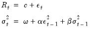 | (27.17) |
you should enter the various parts of your specification:
• Fill in the edit box as
r c
• Enter 1 for the number of ARCH terms, and 1 for the number of GARCH terms, and select GARCH/TARCH.
• Select None for the ARCH-M term.
• Leave blank the Variance Regressors edit box.
To estimate the ARCH(4)-M model:
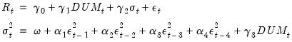 | (27.18) |
you should fill out the dialog in the following fashion:
• Enter the mean equation specification “R C DUM”.
• Enter “4” for the ARCH term and “0” for the GARCH term, and select GARCH (symmetric).
• Select Std. Dev. for the ARCH-M term.
• Enter DUM in the edit box.
Once you have filled in the dialog, click OK to estimate the model. ARCH models are estimated by the method of maximum likelihood, under the assumption that the errors are conditionally normally distributed. Because the variance appears in a non-linear way in the likelihood function, the likelihood function must be estimated using iterative algorithms. In the status line, you can watch the value of the likelihood as it changes with each iteration. When estimates converge, the parameter estimates and conventional regression statistics are presented in the ARCH object window.
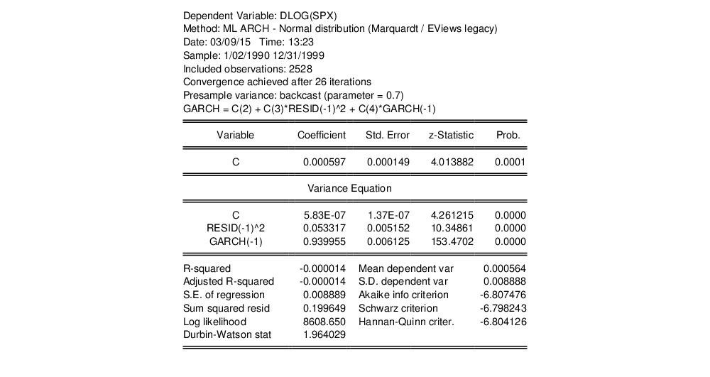
As an example, we fit a GARCH(1,1) model to the first difference of log daily S&P 500 (DLOG(SPX)) in the workfile “Stocks.WF1”, using backcast values for the initial variances and computing Bollerslev-Wooldridge standard errors. The output is presented below:
By default, the estimation output header describes the estimation sample, and the methods used for computing the coefficient standard errors, the initial variance terms, and the variance equation. Also noted is the method for computing the presample variance, in this case backcasting with smoothing parameter

.
The main output from ARCH estimation is divided into two sections—the upper part provides the standard output for the mean equation, while the lower part, labeled “Variance Equation”, contains the coefficients, standard errors, z-statistics and p-values for the coefficients of the variance equation.
The ARCH parameters correspond to

and the GARCH parameters to

in
Equation (27.2). The bottom panel of the output presents the standard set of regression statistics using the residuals from the mean equation. Note that measures such as

may not be meaningful if there are no regressors in the mean equation. Here, for example, the

is negative.
In this example, the sum of the ARCH and GARCH coefficients (

) is very close to one, indicating that volatility shocks are quite persistent. This result is often observed in high frequency financial data.