Estimating a Regression Model
We now estimate a regression model for M1 using data over the period from 1952Q1–1992Q4 and use this estimated regression to construct forecasts over the period 1993Q1–2003Q4. The model specification is given by:
 | (1.1) |
where log(M1) is the logarithm of the money supply, log(GDP) is the log of income, RS is the short term interest rate, and

is the log first difference of the price level (the approximate rate of inflation).
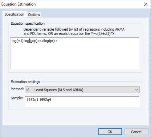
To estimate the model, we will create an equation object. Select from the main menu and choose to open the estimation dialog. Enter the following equation specification:
Here we list the expression for the dependent variable, followed by the expressions for each of the regressors, separated by spaces. The built-in series name C stands for the constant in the regression.
The dialog is initialized to estimate the equation using the LS - Least Squares method for the sample 1952Q1 1996Q4. You should change text in the Sample edit box to “1952Q1 1992Q4” or equivalently “1952 1992” to estimate the equation for the subsample of observations.
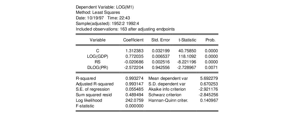
Click OK to estimate the equation using least squares and to display the regression results:
Note that the equation is estimated from 1952Q2 to 1992Q4 since one observation is dropped from the beginning of the estimation sample to account for the DLOG difference term. The estimated coefficients are statistically significant, with
t-statistic values well in excess of 2. The overall regression fit, as measured by the

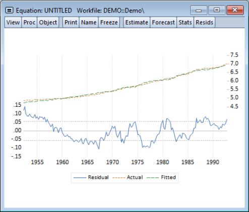
value, indicates a very tight fit. You can select in the equation toolbar to display a graph of the actual and fitted values for the dependent variable, along with the residuals: