Working with the Model Data
When working with a model, much of your time will be spent viewing and modifying the data associated with the model. Before solving the model, you will edit the paths of your exogenous variables or add factors during the forecast period. After solving the model, you will use graphs or tables of the endogenous variables to evaluate the results. Because there is a large amount of data associated with a model, you will also spend time simply managing the data.
Since all the data associated with a model is stored inside standard series in the workfile, you can use all of the usual tools in EViews to work with the data of your model. However, it is often more convenient to work directly from the model window.
Although there are some differences in details, working with the model data generally involves following the same basic steps. You will typically first use the variable view to select the set of variables you would like to work with, then use either the right mouse button menu or the model procedure menu to select the operation to perform.
Because there may be several series in the workfile associated with each variable in the model, you will then need to select the types of series with which you wish to work. The following types will generally be available:
• Actuals: the workfile series with the same name as the variable name. This will typically hold the historical data for the endogenous variables, and the historical data and baseline forecast for the exogenous variables.
• Active: the workfile series that is used when solving the active scenario. For endogenous variables, this will be the series with a name consisting of the variable name followed by the scenario extension. For exogenous variables, the actual series will be used unless it has been overridden. In this case, the exogenous variable will also be the workfile series formed by appending the scenario extension to the variable name.
• Alternate: the workfile series that is used when solving the alternate scenario. The rules are the same as for active.
In the following sections, we discuss how different operations can be performed on the model data from within the variable view.
Editing Data
The easiest way to make simple changes to the data associated with a model is to open a series or group spreadsheet window containing the data, then edit the data by hand.
To open a series window from within the model, simply select the variable using the mouse in the variable view, then use the right mouse button menu to choose , followed by , or . If you select several series before using the option, an unnamed group object will be created to hold all the series.
To edit the data, click the button to make sure the spreadsheet is in edit mode. You can either edit the data directly in levels or use the button to work with a transformed form of the data, such as the differences or percentage changes.
To create a group which allows you to edit more than one of the series associated with a variable at the same time, you can use the procedure discussed below to create a dated data table, then switch the group to spreadsheet view to edit the data.
More complicated changes to the data may require using a genr command to calculate the series by specifying an expression. Click the button from the series window toolbar to call up the dialog, then type in the expression to generate values for the series and set the workfile sample to the range of values you would like to modify.
Displaying Data
The EViews model object provides two main forms in which to display data: as a graph or as a table. Both of these can be generated easily from the model window.
From the variable view, select the variables you wish to display, then use the right mouse button menu or the main menu to select and then or .
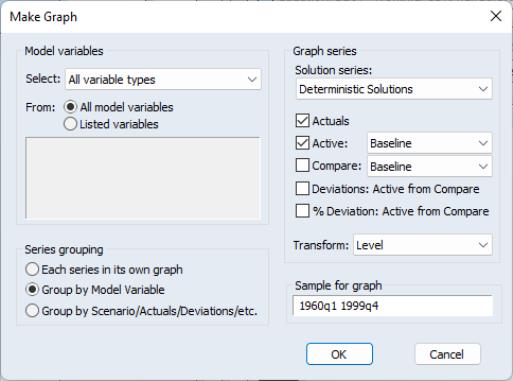
The dialogs for the two procs are almost identical. Here we see the dialog. We saw this dialog earlier in our macro model example. The majority of fields in the dialog control which series you would like the table or graph to contain. At the top left of the graph is the box, which is used to select the set of variables to place in the graph. By default, the table or graph will contain the variables that are currently selected in the variable view. You can expand this to include all model variables, or add or remove particular variables from the list of selected variables using the radio buttons and text box labeled . You can also restrict the set of variables chosen according to variable type using the drop down menu next to . By combining these fields, it is easy to select sets of variables such as all of the endogenous variables of the model, or all of the overridden variables.
Once the set of variables has been determined, it is necessary to map the variable names into the names of series in the workfile. This typically involves adding an extension to each name according to which scenario the data is from and the type of data contained in the series. The options affecting this are contained in the (if you are making a graph) or (if you are making a group/table) box at the right of the dialog.
The box lets you choose which solution results you would like to examine when working with endogenous variables. You can choose from a variety of series generated during deterministic or stochastic simulations.
The series of checkboxes below determine which scenarios you would like to display in the graphs, as well as whether you would like to calculate deviations between various scenarios. You can choose to display the actual series, the series from the active scenario, or the series from an alternate scenario (labeled “Compare”). You can also display either the difference between the active and alternate scenario (labeled “Deviations: Active from Compare”), or the ratio between the active and alternate scenario in percentage terms (labeled “% Deviation: Active from Compare”).
The final field in the or box is the listbox. This lets you apply a transformation to the data similar to the button in the series spreadsheet.
While the deviations and units options allow you to present a variety of transformations of your data, in some cases you may be interested in other transformations that are not directly available. Similarly, in a stochastic simulation, you may be interested in examining standard errors or confidence bounds on the transformed series, which will not be available when you apply transformations to the data after the simulation is complete. In either of these cases, it may be worth adding an identity to the model that generates the series you are interested in examining as part of the model solution.
For example, if your model contains a variable GDP, you may like to add a new equation to the model to calculate the percentage change of GDP:
pgdp = @pch(gdp)
After you have solved the model, you can use the variable PGDP to examine the percentage change in GDP, including examining the error bounds from a stochastic simulation. Note that the cost of adding such identities is relatively low, since EViews will place all such identities in a final recursive block which is evaluated only once after the main endogenous variables have already been solved.
The remaining option, at the bottom left of the dialog, lets you determine how the series will be grouped in the output. The options are slightly different for tables and graphs. For tables, you can choose to either place all series associated with the same model variable together, or to place each series of the same series type together. For graphs, you have the same two choices, and one additional choice, which is to place every series in its own graph.
In the graph dialog, you also have the option of setting a sample for the graph. This is often useful when you are plotting forecast results since it allows you to choose the amount of historical data to display in the graph prior to the forecast results. By default, the sample is set to the workfile sample.
When you have finished setting the options, simply click on to create the new table or graph. All of EViews usual editing features are available to modify the table or graph for final presentation.
Managing Data
When working with a model, you will often create many series in the workfile for each variable, each containing different types of results or the data from different scenarios. The model object provides a number of tools to help you manage these series, allowing you to perform copy, fetch, store and delete operations directly from within the model.
Because the series names are related to the variable names in a consistent way, management tasks can often also be performed from outside the model by using the pattern matching features available in EViews commands (see
Appendix A. “Wildcards”).
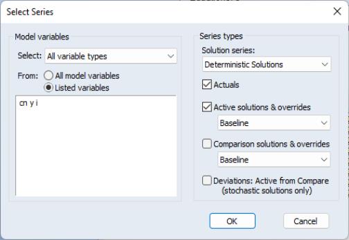
The data management operations from within the model window proceed very similarly to the data display operations. First, select the variables you would like to work with from the variable view, then choose , , or from the right mouse button menu or the object procedures menu. A dialog will appear, similar to the one used when making a table or graph.
In the same way as for the table and graph dialogs, the left side of the dialog is used to choose which of the model variables to work with, while the right side of the dialog is used to select one or more series associated with each variable. Most of the choices are exactly the same as for graphs and tables. One significant difference is that the checkboxes for active and comparison scenarios include exogenous variables only if they have been overridden in the scenario. Unlike when displaying or editing the data, if an exogenous variable has not been overridden, the actual series will not be included in its place. The only way to store, fetch or delete any actual series is to use the checkbox.
After clicking on , you will receive the usual prompts for the store, fetch and delete operations. You can proceed as usual.