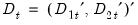
We will work with the standard triangular representation of a regression specification and assume the existence of a single cointegrating vector (Hansen 1992b, Phillips and Hansen 1990). Consider the  dimensional time series vector process
  , with cointegrating equation
dimensional time series vector process , with cointegrating equation
 are deterministic trend regressors and the
  stochastic regressors
  are governed by the system of equations:
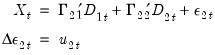
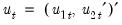
 -vector of
  regressors enter into both the cointegrating equation and the regressors equations, while the
  -vector of
  are deterministic trend regressors which are included in the regressors equations but excluded from the cointegrating equation (if a non-trending regressor such as the constant is present, it is assumed to be an element of
  so it is not in
  ).
).  are strictly stationary and ergodic with zero mean, contemporaneous covariance matrix
  , one-sided long-run covariance matrix
  , and covariance matrix
  , each of which we partition conformably with
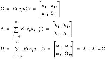
 long-run covariance matrix
  with non-singular sub-matrix
  . Taken together, the assumptions imply that the elements of
  and
and  are I(1) and cointegrated but exclude both cointegration amongst the elements of
  and multicointegration. Discussions of additional and in some cases alternate assumptions for this specification are provided by Phillips and Hansen (1990), Hansen (1992b), and Park (1992).
 in
in
 , and cross-correlation between the cointegrating equation errors and the regressors
  . In the special case where the
  are strictly exogenous regressors so that
  and
and  , the bias, asymmetry, and dependence on non-scalar nuisance parameters vanish, and the SOLS estimator has a fully efficient asymptotic Gaussian mixture distribution which permits standard Wald testing using conventional limiting
  -distributions.
 is no less than the number of stochastic regressors
  . Let
. Let  represent the number of cointegrating regressors less the number of deterministic trend regressors excluded from the cointegrating equation. Then, roughly speaking, when
  , the deterministic trends in the regressors asymptotically dominate the stochastic trend components in the cointegrating equation.
 case.
case.