Estimating a Cointegrating Regression
EViews offers three methods for estimating a single cointegrating vector: Fully Modified OLS (FMOLS), Canonical Cointegrating Regression (CCR), and Dynamic OLS (DOLS). Static OLS is supported as a special case of DOLS. We emphasize again that Johansen’s (1991, 1995) system maximum likelihood approach is discussed in
“Vector Autoregression (VAR) Models”.
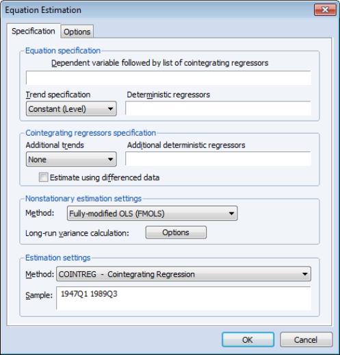
The equation object is used to estimate a cointegrating equation. First, create an equation object, select or then select in the dropdown menu. The dialog will show settings appropriate for your cointegrating regression. Alternately, you may enter the cointreg keyword in the command window to perform both steps.
There are three parts to specifying your equation. First, you should use the first two sections of the dialog ( and ) to specify your triangular system of equations. Second, you will use the section to specify the basic cointegrating regression estimation method. Lastly, you should enter a sample specification, then click on to estimate the equation. (We ignore, for a moment, the options settings on the tab.)
Specifying the Equation
The first two sections of the dialog ( and ) are used to describe your cointegrating and regressors equations.
Equation Specification
The cointegrating equation is described in the section. You should enter the name of the dependent variable,

, followed by a list of cointegrating regressors,

, in the edit field, then use the dropdown to choose from a list of deterministic trend variable assumptions (, , ,). The dropdown menu selections imply trends up to the specified order so that the selection depicted includes a constant and a linear trend term along with the quadratic.
If you wish to add deterministic regressors that are not offered in the pre-specified list to

, you may enter the series names in the edit box.
Cointegrating Regressors Specification
section of the dialog completes the specification of the regressors equations.
First, if there are any

deterministic regressors (regressors that are included in the regressors equations but not in the cointegrating equation), they should be specified here using the dropdown menu or by entering regressors explicitly using the edit field.
Second, you should indicate whether you wish to estimate the regressors innovations

indirectly by estimating the regressors equations in levels and then differencing the residuals or directly by estimating the regressors equations in differences. Check the box for (which is only relevant and only appears if you are estimating your equation using FMOLS or CCR) to estimate the regressors equations in differences.
Specifying an Estimation Method
Once you specify your cointegrating and regressor equations you are ready to describe your estimation method. The EViews equation object offers three methods for estimating a single cointegrating vector: Fully Modified OLS (FMOLS), Canonical Cointegrating Regression (CCR), and Dynamic OLS (DOLS). We again emphasize that Johansen’s (1991, 1995) system maximum likelihood approach is described elsewhere(
“Technical Discussion”).
The section is used to describe your estimation method. First, you should use the dropdown menu to choose one of the three methods. Both the main dialog page and the options page will change to display the options associated with your selection.
Fully Modified OLS
Phillips and Hansen (1990) propose an estimator which employs a semi-parametric correction to eliminate the problems caused by the long run correlation between the cointegrating equation and stochastic regressors innovations. The resulting Fully Modified OLS (FMOLS) estimator is asymptotically unbiased and has fully efficient mixture normal asymptotics allowing for standard Wald tests using asymptotic Chi-square statistical inference.
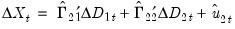
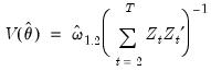
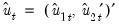
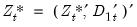
The FMOLS estimator employs preliminary estimates of the symmetric and one-sided long-run covariance matrices of the residuals. Let

be the residuals obtained after estimating
Equation (28.1). The

may be obtained indirectly as

from the levels regressions
 | (28.4) |
or directly from the difference regressions
 | (28.5) |
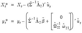
Let

and

be the long-run covariance matrices computed using the residuals
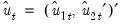
. Then we may define the modified data
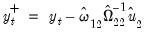 | (28.6) |
and an estimated bias correction term
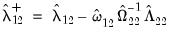 | (28.7) |
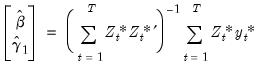
The FMOLS estimator is given by
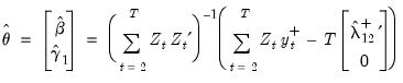 | (28.8) |
where
. The key to FMOLS estimation is the construction of long-run covariance matrix estimators

and

.
Before describing the options available for computing

and

, it will be useful to define the scalar estimator
 | (28.9) |
which may be interpreted as the estimated long-run variance of

conditional on

. We may, if desired, apply a degree-of-freedom correction to

.
Hansen (1992) shows that the Wald statistic for the null hypothesis

 | (28.10) |
with
 | (28.11) |
has an asymptotic

-distribution, where

is the number of restrictions imposed by

. (You should bear in mind that restrictions on the constant term and any other non-trending variables are not testable using the theory underlying
Equation (28.10).)
To estimate your equation using FMOLS, select in the dropdown menu. The main dialog and options pages will change to show the available settings.
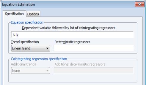
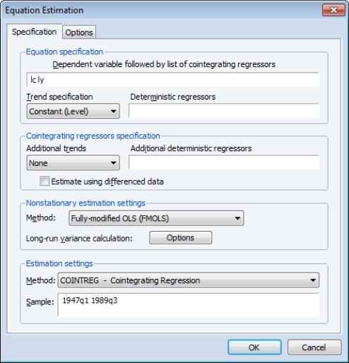
To illustrate the FMOLS estimator, we employ data for (100 times) log real quarterly aggregate personal disposable income (LY) and personal consumption expenditures (LC) for the U.S. from 1947q1 to 1989q3 as described in Hamilton (2000, p. 600, 610) and contained in the workfile “Hamilton_coint.WF1”.
We wish to estimate a model that includes an intercept in the cointegrating equation, has no additional deterministics in the regressors equations, and estimates the regressors equations in non-differenced form.
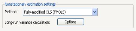
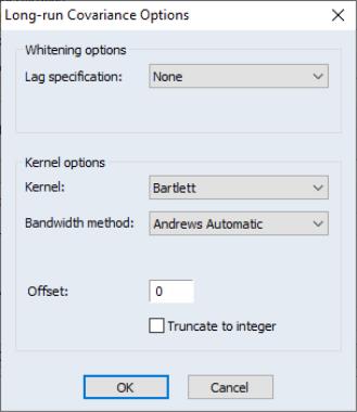
By default, EViews will estimate

and

using a (non-prewhitened) kernel approach with a Bartlett kernel and Newey-West fixed bandwidth. To change the whitening or kernel settings, click on the button and enter your changes in the sub-dialog.
Here we have specified that the long-run variances be computed using a nonparametric method with the Bartlett kernel and a real-valued bandwidth chosen by Andrews’ automatic bandwidth selection method.
In addition, you may use the tab of the dialog to modify the computation of the coefficient covariance. By default, EViews computes the coefficient covariance by rescaling the usual OLS covariances using the

obtained from the estimated

after applying a degrees-of-freedom correction. In our example, we will use the checkbox on the tab (not depicted) to remove the d.f. correction.
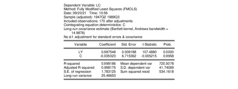
The estimates for this specification are given by:
The top portion of the results describe the settings used in estimation, in particular, the specification of the deterministic regressors in the cointegrating equation, the kernel nonparametric method used to compute the long-run variance estimators

and

, and the no-d.f. correction option used in the calculation of the coefficient covariance. Also displayed is the bandwidth of 14.9878 selected by the Andrews automatic bandwidth procedure.
The estimated coefficients are presented in the middle of the output. Of central importance is the coefficient on LY which implies that the estimated cointegrating vector for LC and LY (1, -0.9875). Note that we present the standard error, t-statistic, and p-value for the constant even though they are not, strictly speaking, valid.
The summary statistic portion of the output is relatively familiar but does require a bit of comment. First, all of the descriptive and fit statistics are computed using the original data, not the FMOLS transformed data. Thus, while the measures of fit and the Durbin-Watson stat may be of casual interest, you should exercise extreme caution in using these measures. Second, EViews displays a “Long-run variance” value which is an estimate of the long-run variance of

conditional on

. This statistic, which takes the value of 25.47 in this example, is the

employed in forming the coefficient covariances, and is obtained from the

and

used in estimation. Since we are not d.f. correcting the coefficient covariance matrix the

reported here is not d.f. corrected.
Once you have estimated your equation using FMOLS you may use the various cointegrating regression equation views and procedures. We will discuss these tools in greater depth in (
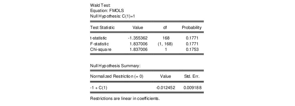
“Working with an Equation”), but for now we focus on a simple Wald test for the coefficients. To test for whether the cointegrating vector is (1, -1), select and enter “C(1)=1” in the dialog. EViews displays the output for the test:
The t-statistic and Chi-square p-values are both around 0.17, indicating that the we cannot reject the null hypothesis that the cointegrating regressor coefficient value is equal to 1.
Note that this Wald test is for a simple linear restriction. Hansen points out that his theoretical results do not directly extend to testing nonlinear hypotheses in models with trend regressors, but EViews does allow tests with nonlinear restrictions since others, such as Phillips and Loretan (1991) and Park (1992) provide results in the absence of the trend regressors. We do urge caution in interpreting nonlinear restriction test results for equations involving such regressors.
Canonical Cointegrating Regression
Park’s (1992) Canonical Cointegrating Regression (CCR) is closely related to FMOLS, but instead employs stationary transformations of the

data to obtain least squares estimates to remove the long run dependence between the cointegrating equation and stochastic regressors innovations. Like FMOLS, CCR estimates follow a mixture normal distribution which is free of non-scalar nuisance parameters and permits asymptotic Chi-square testing.
As in FMOLS, the first step in CCR is to obtain estimates of the innovations
and corresponding consistent estimates of the long-run covariance matrices

and

. Unlike FMOLS, CCR also requires a consistent estimator of the contemporaneous covariance matrix

.
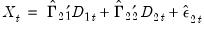
Following Park, we extract the columns of

corresponding to the one-sided long-run covariance matrix of

and (the levels and lags of)

 | (28.12) |
and transform the

using
 | (28.13) |
where the

are estimates of the cointegrating equation coefficients, typically the SOLS estimates used to obtain the residuals

.
The CCR estimator is defined as ordinary least squares applied to the transformed data
 | (28.14) |
where
.
Park shows that the CCR transformations asymptotically eliminate the endogeneity caused by the long run correlation of the cointegrating equation errors and the stochastic regressors innovations, and simultaneously correct for asymptotic bias resulting from the contemporaneous correlation between the regression and stochastic regressor errors. Estimates based on the CCR are therefore fully efficient and have the same unbiased, mixture normal asymptotics as FMOLS. Wald testing may be carried out as in
Equation (28.10) with

used in place of

in
Equation (28.11).
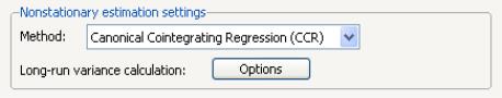
To estimate your equation using CCR, select in the dropdown menu. The main dialog and options pages for CCR are identical to those for FMOLS.
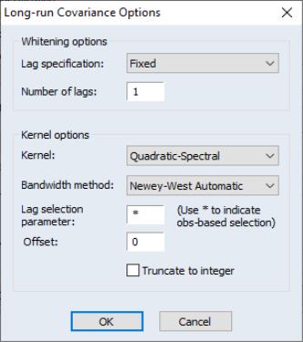
To continue with our consumption and disposable income example, suppose we wish to estimate the same specification as before by CCR, using prewhitened Quadratic-spectral kernel estimators of the long-run covariance matrices. Fill out the equation specification portion of the dialog as before, then click on the button to change the calculation method. Here, we have specified a (fixed lag) VAR(1) for the prewhitening method and have changed our kernel shape to quadratic spectral. Click on to accept the covariance options
Once again go to the tab to turn off d.f. correction for the coefficient covariances so that they match those from FMOLS. Click on again to accept the estimation options.
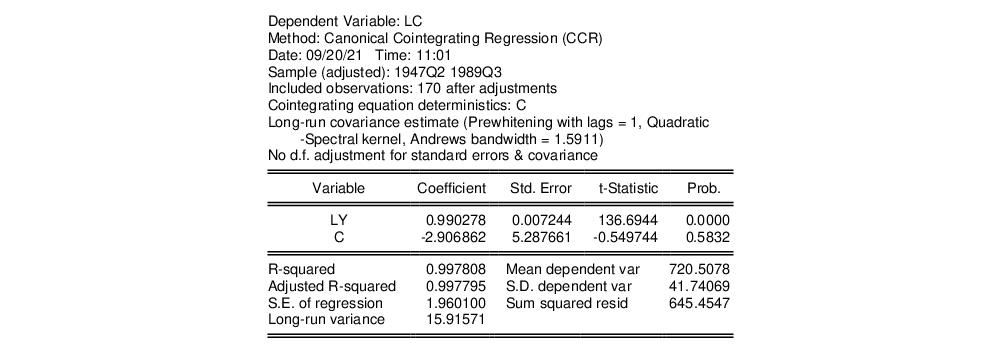
The results are presented below:
The first thing we note is that the VAR prewhitening has a strong effect on the kernel part of the calculation of the long-run covariances, shortening the Andrews optimal bandwidth from almost 15 down to 1.6. Furthermore, as a result of prewhitening, the estimate of the conditional long-run variance changes quite a bit, decreasing from 25.47 to 15.92. This decrease contributes to estimated coefficient standard errors for CCR that are smaller than their FMOLS counterparts. Differences aside, however, the estimates of the cointegrating vector are qualitatively similar. In particular, a Wald test of the null hypothesis that the cointegrating vector is equal to (1, -1) yields a p-value of 0.1814.
Dynamic OLS
A simple approach to constructing an asymptotically efficient estimator that eliminates the feedback in the cointegrating system has been advocated by Saikkonen (1992) and Stock and Watson (1993). Termed Dynamic OLS (DOLS), the method involves augmenting the cointegrating regression with lags
and leads of

so that the resulting cointegrating equation error term is orthogonal to the entire history of the stochastic regressor innovations:
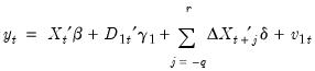 | (28.15) |
Under the assumption that adding

lags and

leads of the differenced regressors soaks up all of the long-run correlation between

and

, least-squares estimates of

using
Equation (28.15) have the same asymptotic distribution as those obtained from FMOLS and CCR.
An estimator of the asymptotic variance matrix of

may be computed by computing the usual OLS coefficient covariance, but replacing the usual estimator for the residual variance of

with an estimator of the long-run variance of the residuals. Alternately, you could compute a robust HAC estimator of the coefficient covariance matrix.
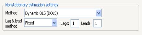
To estimate your equation using DOLS, first fill out the equation specification, then select in the dropdown menu. The dialog will change to display settings for DOLS.
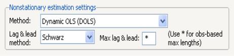
By default, the is with and each set to 1. You may specify a different number of lags or leads or you can use the dropdown to elect automatic information criterion selection of the lag and lead orders by selecting , , or . If you select , EViews will estimate SOLS.
If you select one of the info criterion selection methods, you will be prompted for a maximum lag and lead length. You may enter a value, or you may retain the default entry “*” which instructs EViews to use an arbitrary observation-based rule-of-thumb:
 | (28.16) |
to set the maximum, where

is the number of coefficients in the cointegrating equation. This rule-of-thumb is a slightly modified version of the rule suggested by Schwert (1989) in the context of unit root testing. (We urge careful thought in the use of automatic selection methods since the purpose of including leads and lags is to remove long-run dependence by orthogonalizing the equation residual with respect to the history of stochastic regressor innovations; the automatic methods were not designed to produce this effect.)
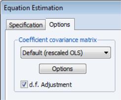
For DOLS estimation we may also specify the method used to compute the coefficient covariance matrix. Click on the tab of the dialog to see the relevant options.
The dropdown menu allows you to choose between the , , , or The default computation method re-scales the ordinary least squares coefficient covariance using an estimator of the long-run variance of DOLS residuals (multiplying by the ratio of the long-run variance to the ordinary squared standard error). Alternately, you may employ a sandwich-style covariance matrix estimator. In both cases, the button may be used to override the default method for computing the long-run variance (non-prewhitened Bartlett kernel and a Newey-West fixed bandwidth). In addition, EViews offers options for estimating the coefficient covariance using the covariance or methods. These methods are offered primarily for comparison purposes.
Lastly, the tab may be used to remove the degree-of-freedom correction that is applied to the estimate of the conditional long-run variance or robust coefficient covariance.
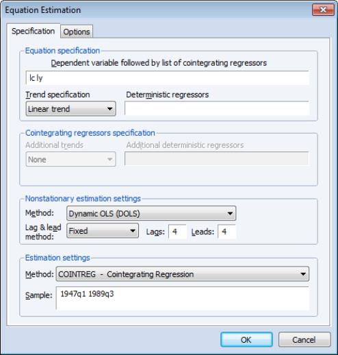
We illustrate the technique by estimating an example from Hamilton (19.3.31, p. 611) using the consumption and income data discussed earlier. The model employs an intercept-trend specification for the cointegrating equation, with no additional deterministics in the regressors equations, and four lags and leads of the differenced cointegrating regressor to eliminate long run correlation between the innovations.
Here, we have entered the cointegrating equation specification in the top portion of the dialog, and chosen as our estimation method, and specified a lag and lead length of 4.
In computing the covariance matrix, Hamilton computes the long-run variance of the residuals using an AR(2) whitening regression with no d.f. correction. To match Hamilton’s computations, we click on the tab to display the covariance. First, turn off the adjustment for degrees of freedom by unchecking the box. Next, with the dropdown set to , click on the button to display the dialogSelect a lag specification of 2, and choose the kernel. Click on to accept the HAC settings, then on again to estimate the equation.
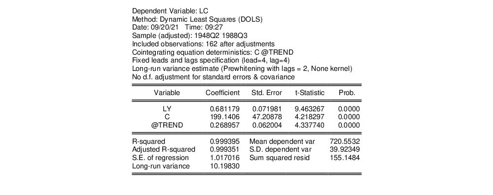
The estimation results are given below:
The top portion describes the settings used in estimation, showing the trend assumptions, the lag and lead specification, and method for computing the long-run variance used in forming the coefficient covariances. The actual estimate of the latter, in this case 10.198, is again displayed in the bottom portion of the output (if you had selected OLS as your coefficient covariance methods, this value would be simply be the ordinary S.E. of the regression; if you had selected White or HAC, the statistic would not have been computed).
The estimated coefficients are displayed in the middle of the output. First, note that EViews does not display the results for the lags and leads of the differenced cointegrating regressors since we cannot perform inference on these short-term dynamics nuisance parameters. Second, the coefficient on the linear trend is statistically different from zero at conventional levels, indicating that there is a deterministic time trend common to both LC and LY. Lastly, the estimated cointegrating vector for LC and LY is (1, -0.6812), which differs qualitatively from the earlier results. A Wald test of the restriction that the cointegrating vector is (1, -1) yields a t-statistic of -4.429, strongly rejecting that null hypothesis.
While EViews does not display the coefficients for the short-run dynamics, the short-run coefficients are used in constructing the fit statistics in the bottom portion of the results view (we again urge caution in using these measures). The short-run dynamics are also used in computing the residuals used by various equation views and procs such as the residual plot or the gradient view.
The short-run coefficients are not included in the representations view of the equation, which focuses only on the estimates for
Equation (28.1). Furthermore, forecasting and model solution using an equation estimated by DOLS are also based on the long-run relationship. If you wish to construct forecasts that incorporate the short-run dynamics, you may use least squares to estimate an equation that explicitly includes the lags and leads of the cointegrating regressors.