Estimation Background
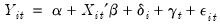
The basic class of models that can be estimated using panel techniques may be written as:
 | (54.35) |
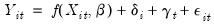
The leading case involves a linear conditional mean specification, so that we have:
 | (54.36) |
where

is the dependent variable, and

is a

‑vector of regressors, and

are the error terms for
cross-sectional units observed for dated periods
. The

parameter represents the overall constant in the model, while the

and

represent cross-section or period specific effects (random or fixed).
Note that in contrast to the pool specifications described in
Equation (52.2), EViews panel equations allow you to specify equations in general form, allowing for nonlinear coefficients mean equations with additive effects. Panel equations do not automatically allow for

coefficients that vary across cross-sections or periods, but you may, of course, create interaction variables that permit such variation.
Other than these differences, the pool equation discussion of
“Estimation Background” applies to the estimation of panel equations. In particular, the calculation of fixed and random effects, GLS weighting, AR estimation, and coefficient covariances for least squares and instrumental variables is equally applicable in the present setting.
Accordingly, the remainder of this discussion will focus on a brief review of the relevant econometric concepts surrounding GMM estimation of panel equations.
GMM Details
The following is a brief review of GMM estimation and dynamic panel estimators. As always, the discussion is merely an overview. For detailed surveys of the literature, see Wooldridge (2002) and Baltagi (2005).
Background
The basic GMM panel estimators are based on moments of the form,
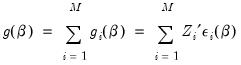 | (54.37) |
where

is a

matrix of instruments for cross-section

, and,
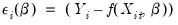 | (54.38) |
In some cases we will work symmetrically with moments where the summation is taken over periods

instead of

.
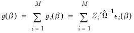
GMM estimation minimizes the quadratic form:
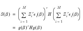 | (54.39) |
with respect to

for a suitably chosen

weighting matrix

.
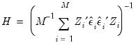
Given estimates of the coefficient vector,

, an estimate of the coefficient covariance matrix is computed as,
 | (54.40) |
where

is an estimator of

, and

is a

derivative matrix given by:
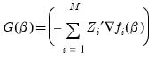 | (54.41) |
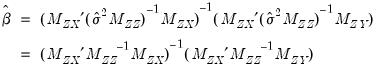
In the simple linear case where
, we may write the coefficient estimator in closed form as,
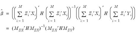 | (54.42) |
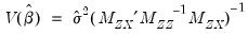
with variance estimator,
 | (54.43) |
for

of the general form:
 | (54.44) |
The basics of GMM estimation involve: (1) specifying the instruments

, (2) choosing the weighting matrix

, and (3) determining an estimator for

.
It is worth pointing out that the summations here are taken over individuals; we may equivalently write the expressions in terms of summations taken over periods. This symmetry will prove useful in describing some of the GMM specifications that EViews supports.
A wide range of specifications may be viewed as specific cases in the GMM framework. For example, the simple 2SLS estimator, using ordinary estimates of the coefficient covariance, specifies:
 | (54.45) |
Substituting, we have the familiar expressions,
 | (54.46) |
and,
 | (54.47) |
Standard errors that are robust to conditional or unconditional heteroskedasticity and contemporaneous correlation may be computed by substituting a new expression for

,
 | (54.48) |
so that we have a White cross-section robust coefficient covariance estimator. Additional robust covariance methods are described in detail in
“Robust Coefficient Covariances”.
In addition, EViews supports a variety of weighting matrix choices. All of the choices available for covariance calculation are also available for weight calculations in the standard panel GMM setting: 2SLS, White cross-section, White period, White diagonal, Cross-section SUR (3SLS), Cross-section weights, Period SUR, Period weights. An additional differenced error weighting matrix may be employed when estimating a dynamic panel data specification using GMM.
The formulae for these weights are follow immediately from the choices given in
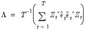
“Robust Coefficient Covariances”. For example, the Cross-section SUR (3SLS) weighting matrix is computed as:
 | (54.49) |
where

is an estimator of the contemporaneous covariance matrix. Similarly, the White period weights are given by:
 | (54.50) |
These latter GMM weights are associated with specifications that have arbitrary serial correlation and time-varying variances in the disturbances.
GLS Specifications
EViews allows you to estimate a GMM specification on GLS transformed data. Note that the moment conditions are modified to reflect the GLS weighting:
 | (54.51) |
Dynamic Panel Data
Consider the linear dynamic panel data specification given by:
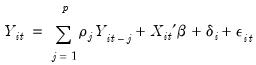 | (54.52) |
First-differencing this specification eliminates the individual effect and produces an equation of the form:
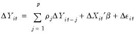 | (54.53) |
which may be estimated using GMM techniques.
Efficient GMM estimation of this equation will typically employ a different number of instruments for each period, with the period-specific instruments corresponding to the different numbers of lagged dependent and predetermined variables available at a given period. Thus, along with any strictly exogenous variables, one may use period-specific sets of instruments corresponding to lagged values of the dependent and other predetermined variables.
Consider, for example, the motivation behind the use of the lagged values of the dependent variable as instruments in
Equation (54.53). If the innovations in the original equation are i.i.d., then in

, the first period available for analysis of the specification, it is obvious that

is a valid instrument since it is correlated with

, but uncorrelated with

. Similarly, in

, both

and

are potential instruments. Continuing in this vein, we may form a set of predetermined instruments for individual

using lags of the dependent variable:
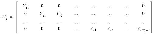 | (54.54) |
Similar sets of instruments may be formed for each predetermined variables.
Assuming that the

are not autocorrelated, the optimal GMM weighting matrix for the differenced specification is given by,
 | (54.55) |
where

is the matrix,
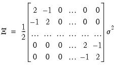 | (54.56) |
and where

contains a mixture of strictly exogenous and predetermined instruments. Note that this weighting matrix is the one used in the one-step Arellano-Bond estimator.
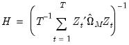
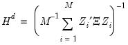
Given estimates of the residuals from the one-step estimator, we may replace the

weighting matrix with one estimated using computational forms familiar from White period covariance estimation:
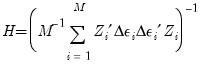 | (54.57) |
This weighting matrix is the one used in the Arellano-Bond two-step estimator.
Lastly, we note that an alternative method of transforming the original equation to eliminate the individual effect involves computing orthogonal deviations (Arellano and Bover, 1995). We will not reproduce the details on here but do note that residuals transformed using orthogonal deviations have the property that the optimal first-stage weighting matrix for the transformed specification is simply the 2SLS weighting matrix:
 | (54.58) |