Specifying a State Space Model in EViews
EViews handles a wide range of single and multiple-equation state space models, providing you with detailed control over the specification of your system equations, covariance matrices, and initial conditions.
The first step in specifying and estimating a state space model is to create a state space object. Select from the main toolbar or type sspace in the command window. EViews will create a state space object and open an empty state space specification window.
There are two ways to specify your state space model. The easiest is to use EViews’ special “auto-specification” features to guide you in creating some of the standard forms for these models. Simply select from the sspace object menu. Specialized dialogs will open to guide you through the specification process. We will describe this method in greater detail in
“Auto-Specification”.
The more general method of describing your state space model uses keywords and text to describe the signal equations, state equations, error structure, initial conditions, and if desired, parameter starting values for estimation. Note that you can insert a state space specification from an existing text file by clicking on the Spec button to display the state space specification, then pressing the right-mouse button menu and selecting
The next section describes the general syntax for the state space object.
Specification Syntax
State Equations
A state equation contains the “@STATE” keyword followed by a valid state equation specification. Bear in mind that:
• Each equation must have a unique dependent variable name; expressions are not allowed. Since EViews does not automatically create workfile series for the states, you may use the name of an existing (non-series) EViews object.
• State equations may not contain signal equation dependent variables, or leads or lags of these variables.
• Each state equation must be linear in the one-period lag of the states. Nonlinearities in the states, or the presence of contemporaneous, lead, or multi-period lag states will generate an error message. We emphasize the point that the one-period lag restriction on states
is not restrictive since higher order lags may be written as new state variables. An example of this technique is provided in the example
“ARMAX(2, 3) with a Random Coefficient”.
• State equations may contain exogenous variables and unknown coefficients, and may be nonlinear in these elements.
In addition, state equations may contain an optional error or error variance specification. If there is no error or error variance, the state equation is assumed to be deterministic. Specification of the error structure of state space models is described in greater detail in
“Errors and Variances”.
Examples
The following two state equations define an unobserved error with an AR(2) process:
@state sv1 = c(2)*sv1(-1) + c(3)*sv2(-1) + [var = exp(c(5))]
@state sv2 = sv1(-1)
The first equation parameterizes the AR(2) for SV1 in terms of an AR(1) coefficient, C(2), and an AR(2) coefficient, C(3). The error variance specification is given in square brackets. Note that the state equation for SV2 defines the lag of SV1 so that SV2(-1) is the two period lag of SV1.
Similarly, the following are valid state equations:
@state sv1 = sv1(-1) + [var = exp(c(3))]
@state sv2 = c(1) + c(2)*sv2(-1) + [var = exp(c(3))]
@state sv3 = c(1) + exp(c(3)*x/z) + c(2)*sv3(-1) + [var = exp(c(3))]
describing a random walk, and an AR(1) with drift (without/with exogenous variables).
The following are not valid state equations:
@state exp(sv1) = sv1(-1) + [var = exp(c(3))]
@state sv2 = log(sv2(-1)) + [var = exp(c(3))]
@state sv3 = c(1) + c(2)*sv3(-2) + [var=exp(c(3))]
since they violate at least one of the conditions described above (in order: expression for dependent state variable, nonlinear in state, multi-period lag of state variables).
Observation/Signal Equations
By default, if an equation specification is not specifically identified as a state equation using the “@STATE” keyword, it will be treated by EViews as an observation or signal equation. Signal equations may also be identified explicitly by the keyword “@SIGNAL”. There are some aspects of signal equation specification to keep in mind:
• Signal equation dependent variables may involve expressions.
• Signal equations may not contain current values or leads of signal variables. You should be aware that any lagged signals are treated as predetermined for purposes of multi-step ahead forecasting (for discussion and alternative specifications, see Harvey 1989, p. 367-368).
• Signal equations must be linear in the contemporaneous states. Nonlinearities in the states, or the presence of leads or lags of states will generate an error message. Again, the restriction that there are no state lags is not restrictive since additional deterministic states may be created to represent the lagged values of the states.
• Signal equations may have exogenous variables and unknown coefficients, and may be nonlinear in these elements.
Signal equations may also contain an optional error or error variance specification. If there is no error or error variance, the equation is assumed to be deterministic. Specification of the error structure of state space models is described in greater detail in
“Errors and Variances”.
Examples
The following are valid signal equation specifications:
log(passenger) = c(1) + c(3)*x + sv1 + c(4)*sv2
@signal y = sv1 + sv2*x1 + sv3*x2 + sv4*y(-1) + [var=exp(c(1))]
z = sv1 + sv2*x1 + sv3*x2 + c(1) + [var=exp(c(2))]
The following are invalid equations:
log(passenger) = c(1) + c(3)*x + sv1(-1)
@signal y = sv1*sv2*x1 + [var = exp(c(1))]
z = sv1 + sv2*x1 + z(1) + c(1) + [var = exp(c(2))]
since they violate at least one of the conditions described above (in order: lag of state variable, nonlinear in a state variable, lead of signal variable).
Errors and Variances
While EViews always adds an implicit error term to each equation in an equation or system object, the handling of error terms differs in a sspace object. In a sspace object, the equation specifications in a signal or state equation do not contain error terms unless specified explicitly.
The easiest way to add an error to a state space equation is to specify an implied error term using its variance. You can simply add an error variance expression, consisting of the keyword “VAR” followed by an assignment statement (all enclosed in square brackets), to the existing equation:
@signal y = c(1) + sv1 + sv2 + [var = 1]
@state sv1 = sv1(-1) + [var = exp(c(2))]
@state sv2 = c(3) + c(4)*sv2(-1) + [var = exp(c(2)*x)]
The specified variance may be a known constant value, or it can be an expression containing unknown parameters to be estimated. You may also build time-variation into the variances using a series expression. Variance expressions may not, however, contain state or signal variables.
While straightforward, this direct variance specification method does not admit correlation between errors in different equations (by default, EViews assumes that the covariance between error terms is 0). If you require a more flexible variance structure, you will need to use the “named error” approach to define named errors with variances and covariances, and then to use these named errors as parts of expressions in the signal and state equations.
The first step of this general approach is to define your named errors. You may declare a named error by including a line with the keyword “@ENAME” followed by the name of the error:
@ename e1
@ename e2
Once declared, a named error may enter linearly into state and signal equations. In this manner, one can build correlation between the equation errors. For example, the errors in the state and signal equations in the sspace specification:
y = c(1) + sv1*x1 + e1
@state sv1 = sv1(-1) + e2 + c(2)*e1
@ename e1
@ename e2
are, in general, correlated since the named error E1 appears in both equations.
In the special case where a named error is the only error in a given equation, you can both declare and use the named residual by adding an error expression consisting of the keyword “ENAME” followed by an assignment and a name identifier:
y = c(1) + sv1*x1 + [ename = e1]
@state sv1 = sv1(-1) + [ename = e2]
The final step in building a general error structure is to define the variances and covariances associated with your named errors. You should include a sspace line comprised of the keyword “@EVAR” followed by an assignment statement for the variance of the error or the covariance between two errors:
@evar cov(e1, e2) = c(2)
@evar var(e1) = exp(c(3))
@evar var(e2) = exp(c(4))*x
The syntax for the @EVAR assignment statements should be self-explanatory. Simply indicate whether the term is a variance or covariance, identify the error(s), and enter the specification for the variance or covariance. There should be a separate line for each named error covariance or variance that you wish to specify. If an error term is named, but there are no corresponding “VAR=” or @EVAR specifications, the missing variance or covariance specifications will remain at the default values of “NA” and “0”, respectively.
As you might expect, in the special case where an equation contains a single error term, you may combine the named error and direct variance assignment statements:
@state sv1 = sv1(-1) + [ename = e1, var = exp(c(3))]
@state sv2 = sv2(-1) + [ename = e2, var = exp(c(4))]
@evar cov(e1, e2) = c(5)
A Note on Correlated Errors
We caution that you should think very carefully about the timing of your errors if you allow for correlation between errors in the state and signal equations. The timing in the signal equation and state equation updates specified in
Equation (50.2) and
Equation (50.1), implies that correlation between the signal and state errors is defined to be between the errors in the signal at time

, and the errors in the states dated in

. This timing may not be what you intend. To allow for correlation in the contemporaneous states and signals in time

, you will need to specify errors in the lagged states, and define correlation between the lagged state errors and the errors in the signal equation.
Specification Examples
ARMAX(2, 3) with a Random Coefficient
We can use the syntax described above to define an ARMAX(2,3) with a random coefficient for the regression variable X:
y = c(1) + sv5*x + sv1 + c(4)*sv2 + c(5)*sv3 + c(6)*sv4
@state sv1 = c(2)*sv1(-1) + c(3)*sv2(-1) + [var=exp(c(7))]
@state sv2 = sv1(-1)
@state sv3 = sv2(-1)
@state sv4 = sv3(-1)
@state sv5 = sv5(-1) + [var=3]
The AR coefficients are parameterized in terms of C(2) and C(3), while the MA coefficients are given by C(4), C(5) and C(6). The variance of the innovation is restricted to be a positive function of C(7). SV5 is the random coefficient on X, with variance restricted to be 3.
Recursive and Random Coefficients
The following example describes a model with one random coefficient (SV1), one recursive coefficient (SV2), and possible correlation between the errors for SV1 and Y:
y = c(1) + sv1*x1 + sv2*x2 + [ename = e1, var = exp(c(2))]
@state sv1 = sv1(-1) + [ename = e2, var = exp(c(3)*x)]
@state sv2 = sv2(-1)
@evar cov(e1,e2) = c(4)
The variances and covariances in the model are parameterized in terms of the coefficients C(2), C(3) and C(4), with the variances of the observed Y and the unobserved state SV1 restricted to be non-negative functions of the parameters.
Parameter Starting Values
Unless otherwise instructed, EViews will initialize all parameters to the current values in the corresponding coefficient vector or vectors. As in the system object, you may override this default behavior by specifying explicitly the desired values of the parameters using a PARAM or @PARAM statement. For additional details, see
“Starting Values”.
Specifying Initial Conditions
By default, EViews will handle the initial conditions for you. For some stationary models, steady-state conditions allow us to solve for the values of

and

. For cases where it is not possible to solve for the initial conditions, EViews will treat the initial values as diffuse, setting

, and

to an arbitrarily high number to reflect our uncertainty about the values (see
“Technical Discussion”).
You may, however have prior information about the values of

and

. In this case, you can create a vector or matrix that contains the appropriate values, and use the “@MPRIOR” or “@VPRIOR” keywords to perform the assignment.
To set the initial states, enter “@MPRIOR” followed by the name of a vector object. The length of the vector object must match the state dimension. The order of elements should follow the order in which the states were introduced in the specification screen.
@mprior v1
@vprior m1
To set the initial state variance matrix, enter “@VPRIOR” followed by the name of a sym object (note that it must be a sym object, and not an ordinary matrix object). The dimensions of the sym must match the state dimension, with the ordering following the order in which the states appear in the specification. If you wish to set a specific element to be diffuse, simply assign the element the “NA” missing value. EViews will reset all of the corresponding variances and covariances to be diffuse.
For example, suppose you have a two equation state space object named SS1 and you want to set the initial values of the state vector and the state variance matrix as:
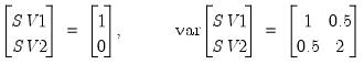 | (50.17) |
First, create a named vector object, say SVEC0, to hold the initial values. Click , choose Matrix-Vector-Coef and enter the name SVEC0. Click OK, and then choose the type Vector and specify the size of the vector (in this case 2 rows). When you click OK, EViews will display the spreadsheet view of the vector SVEC0. Click the button to toggle on edit mode and type in the desired values. Then create a named symmetric matrix object, say SVAR0, in an analogous fashion.
Alternatively, you may find it easier to create and initialize the vector and matrix using commands. You can enter the following commands in the command window:
vector(2) svec0
svec0.fill 1, 0
sym(2) svar0
svar0.fill 1, 0.5, 2
Then, simply add the lines:
@mprior svec0
@vprior svar0
to your sspace object by editing the specification window. Alternatively, you can type the following commands in the command window:
ss1.append @mprior svec0
ss1.append @vprior svar0
For more details on matrix objects and the
fill and
append commands, see
“Matrix Language”.
Specification Views
State space models may be very complex. To aid you in examining your specification, EViews provides views which allow you to view the text specification in a more compact form, and to examine the numerical values of your system matrices evaluated at current parameter values.
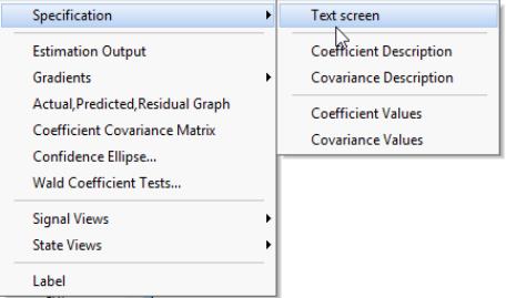
Click on the menu and select The following Specification views are always available, regardless of whether the sspace has previously been estimated:
• . This is the familiar text view of the specification. You should use this view when you create or edit the state space specification. This view may also be accessed by clicking on the button on the sspace toolbar.
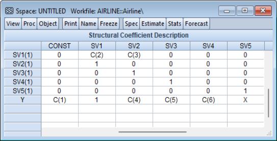
• . Text description of the structure of your state space specification. The variables on the left-hand side, representing

and

, are expressed as linear functions of the state variables

, and a remainder term CONST. The elements of the matrix are the corresponding coefficients. For example, the ARMAX example has the following Coefficient Description view:
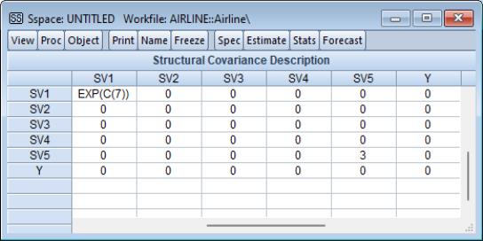
• . Text description of the covariance matrix of the state space specification. For example, the ARMAX example has the following Covariance Description view:
• . Numeric description of the structure of the signal and the state equations evaluated at current parameter values. If the system coefficient matrix is time-varying, EViews will prompt you for a date/observation at which to evaluate the matrix.
• . Numeric description of the structure of the state space specification evaluated at current parameter values. If the system covariance matrix is time-varying, EViews will prompt you for a date/observation at which to evaluate the matrix.
Auto-Specification
To aid you in creating a state space specification, EViews provides you with “auto-specification” tools which will create the text representation of a model that you specify using dialogs. This tool may be very useful if your model is a standard regression with fixed, recursive, and various random coefficient specifications, and/or your errors have a general ARMA structure.
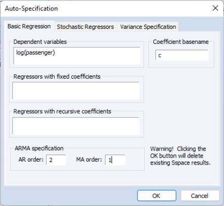
When you select from the menu, EViews opens a three tab dialog. The first tab is used to describe the basic regression portion of your specification. Enter the dependent variable, and any regressors which have fixed or recursive coefficients. You can choose which COEF object EViews uses for indicating unknowns when setting up the specification. At the bottom, you can specify an ARMA structure for your errors. Here, we have specified a simple ARMA(2,1) specification for LOG(PASSENGER).
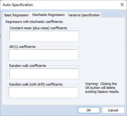
The second tab of the dialog is used to add any regressors which have random coefficients. Simply enter the appropriate regressors in each of the four edit fields. EViews allows you to define regressors with any combination of constant mean, AR(1), random walk, or random walk (with drift) coefficients.
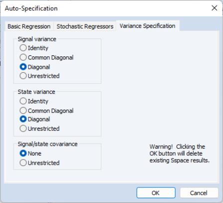
Lastly, the dialog allows you to choose between basic variance structures for your state space model. Click on the tab, and choose between an matrix, (diagonal with common variances), , or general () variance matrix for the signals and for the states. The dialog also allows you to allow the signal equation(s) and state equations(s) to have non-zero error covariances.
We emphasize the fact that your sspace object is not restricted to the choices provided in this dialog. If you find that the set of specifications supported by is too restrictive, you may use it the dialogs as a tool to build a basic specification, and then edit the specification to describe your model.
Estimating a State Space Model
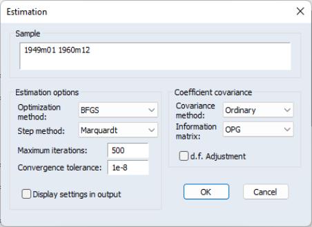
Once you have specified a state space model and verified that your specification is correct, you are ready to estimate the model. To open the estimation dialog, simply click on the button on the toolbar or select
As with other estimation objects, EViews allows you to set the estimation sample, optimization and coefficient covariance methods, the maximum number of iterations, convergence tolerance, the estimation algorithm, derivative settings and whether to display the starting values.
The default optimization method for new sspace objects is BFGS, but you may also select Newton-Raphson, OPG - BHHH, or EViews legacy. For non-legacy estimation, the allows you to choose between the default , , and Line search determined steps.
The default employs the inverse of the matrix specified in the dropdown menu. Alternately, you may compute the sandwich covariance by selecting in the menu.
The outer-product of the gradients () is the default information matrix estimator. If you are performing non-legacy optimization, you may use the observed Hessian by selecting .
The default settings should provide a good start for most problems; if you choose to change the settings, see
“Setting Estimation Options” for related discussion of estimation options.
When you click on , EViews will begin estimation using the specified settings.
There are two additional things to keep in mind when estimating your model:
• Although the EViews Kalman filter routines will automatically handle any missing values in your sample, EViews does require that your estimation sample be contiguous, with no gaps between successive observations.
• If there are no unknown coefficients in your specification, you will still have to “estimate” your sspace to run the Kalman filter and initialize elements that EViews needs in order to perform further analysis.
Interpreting the estimation results
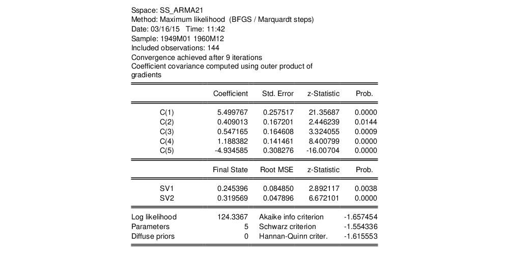
After you choose the variance options and click OK, EViews presents the estimation results in the state space window. For example, if we specify an ARMA(2,1) for the log of the monthly international airline passenger totals from January 1949 to December 1960 (from Box and Jenkins, 1976, series G, p. 531):
log(passenger) = c(1) + sv1 + c(4)*sv2
@state sv1 = c(2)*sv1(-1) + c(3)*sv2(-1) + [var=exp(c(5))]
@state sv2 = sv1(-1)
and estimate the model, EViews will display the estimation output view:
The bulk of the output view should be familiar from other EViews estimation objects. The information at the top describes the basics of the estimation: the name of the sspace object, estimation method, the date and time of estimation, sample and number of objects in the sample, convergence information, and the coefficient estimates. The bottom part of the view reports the maximized log likelihood value, the number of estimated parameters, and the associated information criteria.
Some parts of the output, however, are new and may require discussion. The bottom section provides additional information about the handling of missing values in estimation. “Likelihood observations” reports the actual number of observations that are used in forming the likelihood. This number (which is the one used in computing the information criteria) will differ from the “Included observations” reported at the top of the view when EViews drops an observation from the likelihood calculation because all of the signal equations have missing values. The number of omitted observations is reported in “Missing observations”. “Partial observations” reports the number of observations that are included in the likelihood, but for which some equations have been dropped. “Diffuse priors” indicates the number of initial state covariances for which EViews is unable to solve and for which there is no user initialization. EViews’ handling of initial states and covariances is described in greater detail in
“Initial Conditions”.
EViews also displays the final one-step ahead values of the state vector,

, and the corresponding RMSE values (square roots of the diagonal elements of

). For settings where you may care about the entire path of the state vector and covariance matrix, EViews provides you with a variety of views and procedures for examining the state results in greater detail.