Working with Smooth Threshold Equations
The smooth threshold equation estimated by EViews is a particular nonlinear regression specification. Accordingly, EViews supports the most of the views and procs for a nonlinear regression equation, alongside a number of tools that are specific to STR regression.
We describe below the basics of working with your STR, highlighting views and procs that are specific to STR and those which differ substantively from the standard nonlinear regression implementation.
Estimation Output
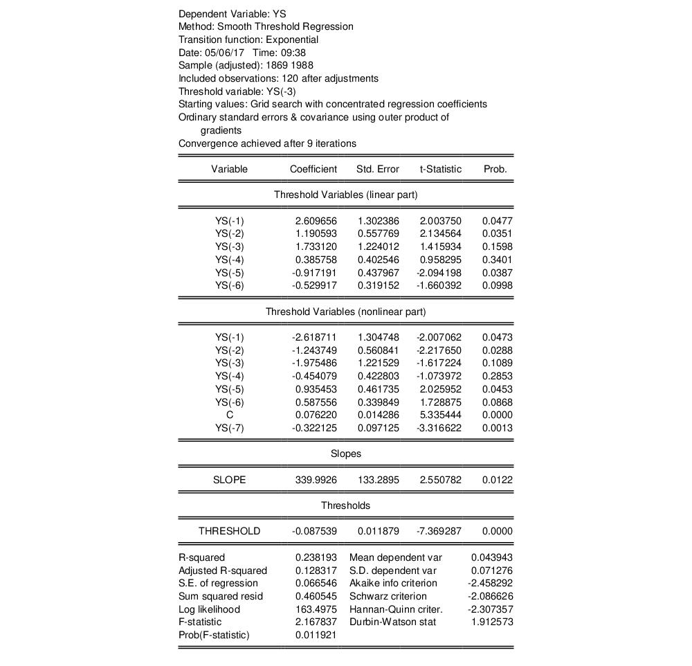
Following estimation, EViews displays the STR output. For example, we might have:
The top portion of the output displays the dependent variable, method, date, sample information, description of the threshold specification, and information about the estimation procedure. In this example, we see that the logistic STR (LSTR) is self-exciting, as the threshold variable is the first lag of the dependent variable. Estimation converged after 9 iterations, from employed starting values obtained from grid search after concentrating out the regression coefficients. The coefficient standard errors and covariance uses the standard inverse outer product of the gradients times the d.f. corrected estimator of the residual variance.
The middle part of the output displays coefficient values and associated statistics for both the base (linear part) and alternative (nonlinear par) of the specification. EViews also reports the estimates slope (

) and threshold (

) parameters.
The bottom portion of the output contains the usual summary statistics.Most of the summary statistics are self-explanatory. Note that the

-square, the
F-statistic, and the corresponding probability are all based on a comparison with the no threshold, constant only linear model.
Equation Views and Procs
The views and procs for smooth threshold equations parallel those in nonlinear least squares regression, with some additions as documented below. We will not discuss familiar residuals and residual diagnostics, gradients and derivatives, and coefficient covariance views and procedures, but will focus instead of views which are new or differ for equations estimated by STR.
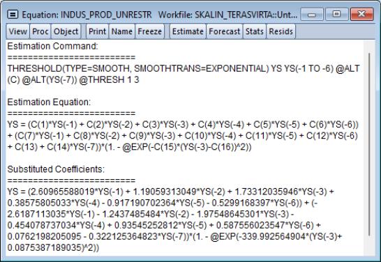
Representations View
As always, the representations view () shows the estimation command. In addition, the view depicts the estimation equation and substituted coefficients sections which show the nonlinear regression specification which combines the coefficients from different regimes with the slope and threshold variable into a single equation.
Note that estimating the estimation equation via ordinary least squares will produce the same coefficients as the estimated smooth threshold model.
Threshold Smoothing Weights
The threshold function occupies a central place in the specification of STR models. Accordingly, EViews offers easy-to-use tools for examining the weights associated with your estimated equation
Threshold Weights View
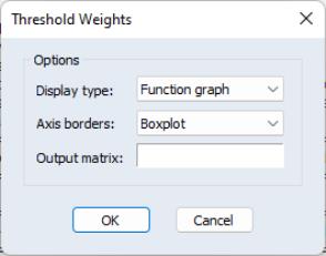
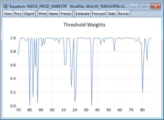
The threshold weights view allows you to examine at the shape of the smoothing function or the values of the smoothing weights for each observation in the estimation sample.
Select to display the dialog:
By default, this view will display a showing the values returned by

for various values of

, and will display that summarize the distribution of the observed individual threshold values and smoothing weights along borders of graph.
You may use the dropdown menu to instead display a , , or for the individual weights.
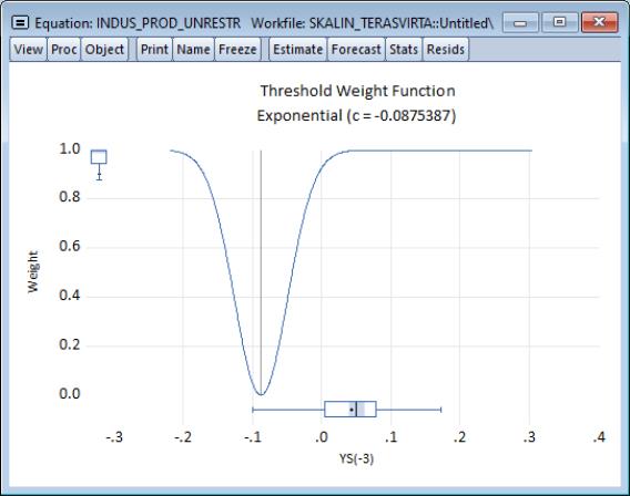
• The default display will show the shape of the estimated smoothing function.
When displaying a , you may use the dropdown to display summary graphs for the individual weights along the axis of the graph. You may choose to display a , , or a , or .
You may save the function plot data to a matrix in the workfile by providing the name of a new or existing in the corresponding edit field.
• The and display the individual weight data for each observation in graph or spreadsheet form.
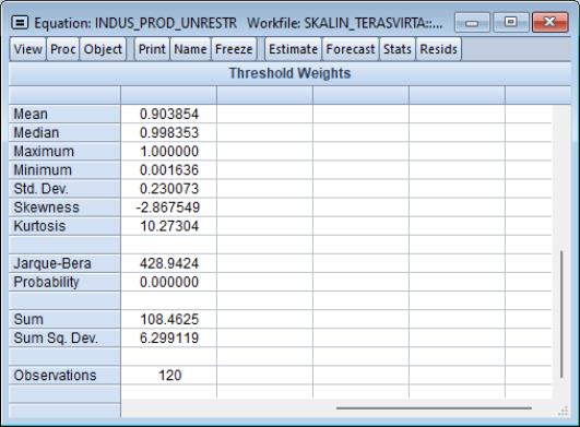
• The setting shows descriptive statistics for the individual weights.
Save Threshold Weights Proc
The threshold weights proc lets you save the individual threshold weight values as a series in your workfile.
To save a series in the workfile containing the individual smoothing weights, click on and enter a name for the weight series in the edit field. Click on to save the weight series.
Model Selection Summary
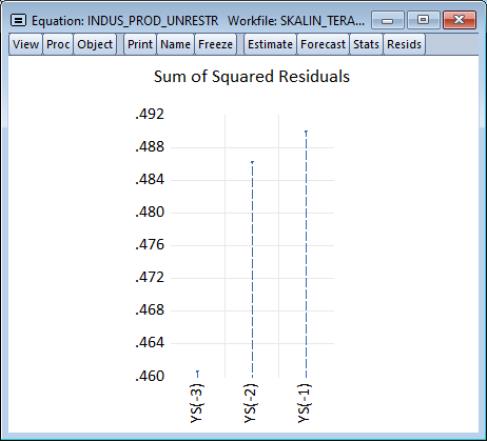
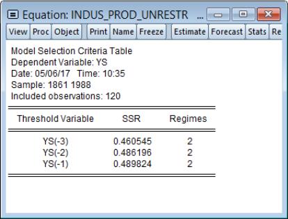
If you specify more than one potential threshold variable, EViews will estimate a STR model using each candidate threshold variable and will choose the specification that minimizes the sum-of-squares. You may examine the results of this model selection procedure using the model selection views.
To display a graph of the results, ordered from best to worst, select :
To display a table of the results, click on :
Stability Diagnostics
EViews provides easy-to-use tests for linearity against STR alternatives as well as tests for misspecification of the STR model by considering the hypotheses of no remaining nonlinearity, of parameter constancy, of no serial correlation, and of homoskedasticity,
Linearity Testing
We may rewrite the basic form of the STR specification
Equation (36.3) as:
 | (36.12) |
where

. For convenience, we will assume that
. This is not an important restriction as the functions above may be modified slightly to enforce this condition.
We can test for linearity under the null hypothesis using either

or

, and as it is more convenient to test for

, the literature focuses on this restriction. Note, however, that under the null hypothesis, the parameters

and

are not identified, so that standard theory cannot be used to obtain the null distribution of the test statistic.
Luukkonen, Saikkonen, and Teräsvirta (1988) propose an approach which replaces

by a Taylor series expansion which is estimable under the null. The resulting test procedure involves taking the linear portion of the model and adding terms representing the interaction of the linear regressors with the polynomial terms in the Taylor expansion and then testing for the statistical significance of sets of the interaction coefficients.
It is worth noting that the resulting Taylor series expansion will differ depending on the form for

and that the specific terms of the Taylor expansion that are asymptotically relevant under the alternative differ across

. These differences allow us to use the probabilities of rejection of various null hypothesis to discriminate between alternative choices for

.
There is a large literature discussing the properties of these tests, offering elaboration and various refinements. For details, see Teräsvirta (1994), Eitrheim and Teräsvirta (1996), Escribano and Jorda (1999), van Dijk, Teräsvirta, and Franses (2002).
To perform these tests, simply click on . EViews will perform linearity tests against nonlinear alternatives using the selected threshold variable.
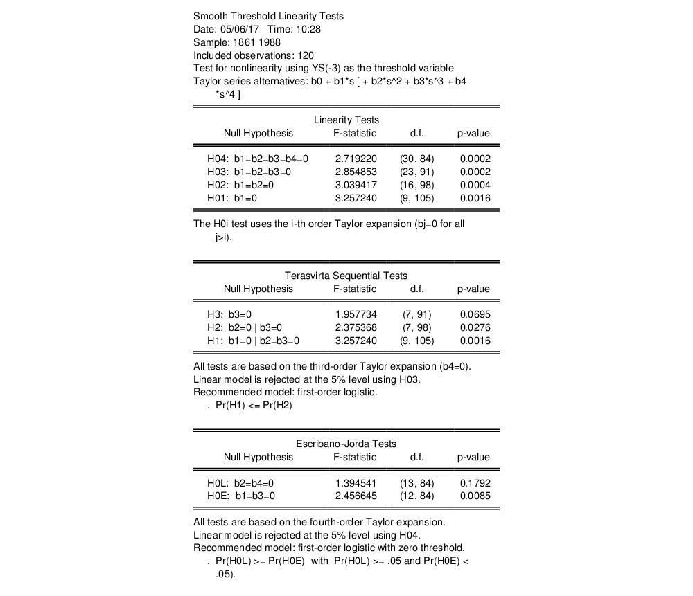
EViews displays results from three different sets of tests.
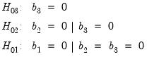
• The Luukkonen, Saikkonen, and Teräsvirta linearity tests at the top of the output are joint hypothesis test for significance of the elements of the Taylor expansion.
The listed hypothesis refers to the coefficients of the expansion under test assuming that the higher order terms are restricted to zero. Imposing these restrictions may produce tests with higher power.
For example, the H02 null hypothesis tests b1=b2=0 assuming that b3=b4=0.
• The Teräsvirta tests are a sequential set of general-to-specific tests for terms of the Taylor expansion that allow for transition function selection. Following Teräsvirta, EViews carries out the three tests in the following sequence:
 | (36.13) |
If the null of linearity is rejected, we may use the results to determine a preferred transition function. A useful rule for discriminating between ESTAR and LSTAR models is to select the ESTAR model if the p-value for H2 is smallest, otherwise the LSTAR model is to be preferred.
• The Escribano-Jorda tests use the different properties of the Taylor expansion both to test for nonlinearity and to discriminate between alternative choices for

. The HOL test evaluates linearity against a logistic alternative, while the HOE test compares linearity to an exponential alternative.
Note that EViews computes the F-statistic forms of all of these tests.
Further, note that we assume that the threshold variable is the one used in estimation of your STR model. Thus, EViews implementation does not allow for the forms of the linearity test where one tests against multiple thresholds.
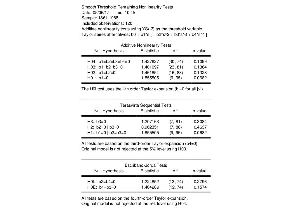
Remaining Nonlinearity Tests
Given estimation of a two-regime STR model we may wish to test for whether there is additional unmodeled nonlinearity. One popular approach is to test the estimated model against a model with additional regimes. The testing methodology is analogous to the linearity tests outlined above (
“Linearity Testing”) in which we consider a Taylor series expansion of the transition weighting function, and then test for the significance of interactions with the variables of the specification.
Following the discussion in van Dijk, Teräsvirta, and Franses (2002) we distinguish between two forms of the test, the additive and the encapsulated tests, which offer different specifications of the multiple regime alternative.
Additive Multiple Regime STR (AMRSTR)
We may specify a three regime model by adding a second nonlinear component, as in:
 | (36.14) |
Eitrheim and Terasvirta (1998) develop LM tests to test the two-regime LSTAR model against this alternative. The test involves expanding the

function in a third-order Taylor expansion and then performing a standard hypothesis test on polynomial terms interacted with

.
To perform a remaining nonlinearity test against this three regime alternative, you should click on :
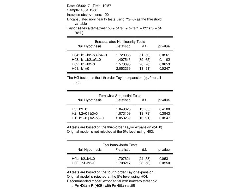
Multiple Regime STR (MRSTR)
The Multiple Regime STR model encapsulates a STR model in a higher regime STR model. For our three regime alternative, we have
 | (36.15) |
Note that both the linear and nonlinear terms in the first node appear in the second node, and that we have kept the non-varying regressors outside of the second nonlinear node.
van Dijk and Franses (1999) develop an LM test in this framework for testing the null of the two regime LSTAR model against the MRSTAR alternative.
To perform a remaining nonlinearity test against the encapsulated three regime alternative, select :
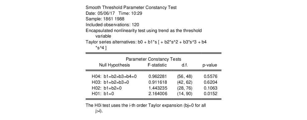
Parameter Constancy Test
One interesting variant of the STR model is the time-varying coefficient specification which is obtained by choosing time to be the threshold variable. This model allows for structural instability in which regression parameters evolve smoothly over time.
If we take the test methodology outlined in
“Linearity Testing” and test against the Taylor series expansion using the threshold variable

, we obtain a test for parameter constancy.
To perform this test, select :
Note that EViews only performs the first form of the linearity test and not the remaining tests which discriminate between threshold variables. The latter may, however, be obtained by first estimating the STR time-varying coefficient specification and performing the standard linearity test on that equation.
Forecasting
Static and one-step ahead forecasting from an STR estimated equation is straightforward. These simple forecasts all involve conditioning on the observed regressors (including any lagged endogenous regressors) and using the estimated specification to evaluate the forecast.
n-step ahead forecasting of STAR and other nonlinear dynamic models is considerably more difficult. For these dynamic forecasting problems, EViews computes the forecasts by stochastic simulation, with the forecasts and forecast standard errors obtained from the sample average and the standard deviation of the simulated values.
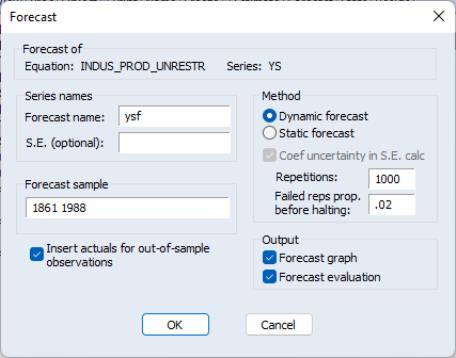
To perform the forecast simulation, click on the button on the equation toolbar or select from the equation menu to display the dialog.
If your equation has dynamic components, you will offered a choice between producing a or a . If you select , EViews will display options for choosing the number of simulation , and for specifying a the simulation.