Background
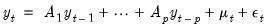
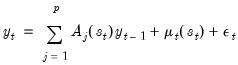
We offer a brief background for switching VAR models. Recall the standard

-dimensional, VAR(
p) process
 | (49.1) |
where
• 
is a

vector of endogenous variables,
• 
are

matrices of lag coefficients to be estimated,
• 
is a

vector of intercepts,
• 
is a

white noise innovation process, with

,
, and

for

.
The vector of innovations are contemporaneously correlated with full rank matrix

, but are uncorrelated with their leads and lags of the innovations and assumed to be uncorrelated with all of the right-hand side variables.
Switching Specification
Following Krolzig, we modify
Equation (49.1) to allow for regime change so that

follows a VAR process that depends on the value of an unobserved discrete state variable

. We assume there are
possible regimes, and we are said to be in regime

in period

when

.
As in Krolzig, the VAR regime dependence is assumed to take one of two forms:
• switching intercept (SI):
 | (49.2) |
• switching mean (SM):
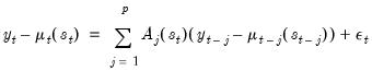 | (49.3) |
Regime change in the SI model produces smooth changes in the time series, while the SM specification produces an immediate jump in mean.
Further, we will assume that the errors are distributed as
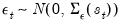
for
, with density function
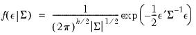 | (49.4) |
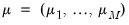
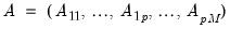
Common practice divides the parameters in the VAR specification into three groups: the intercept parameters

, the endogenous variables parameters

, the error variance parameters

, Typically, only a subset of the groups is allowed to vary across regimes. For example, a common restriction is that only the intercepts, or only the intercepts and the error variances are regime specific.
Lastly, we may allow for exogenous variables by defining the intercepts as functions of exogenous variables and coefficients:
 | (49.5) |
• 
is a

matrix of exogenous variable coefficients to be estimated,
• 
is a

vector of exogenous variables,
so the

are parameterized in terms of exogenous variable parameters
. The remainder of our discussion will be in terms of

, but the analysis can extend to underlying

parameters.
Regime Dependence
Central to the analysis of a switching VAR model is the notion that error term depends on an unobserved state variable. The nature of this state dependence differs dramatically between the switching intercept (SI) and switching mean (SM) specifications introduced earlier.
This difference creates some notational challenges. To facilitate discussion, the remainder of our discussion will organized around a new variable

that is defined in terms of current and lagged

and has

possible states.
We define

for both specifications in the discussion below.
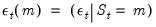
Switching Intercept (SI) Specification
We may use
Equation (49.2) to obtain an expression for the switching intercept error in terms of the observed data and current unobserved state:
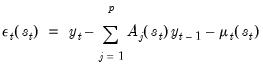 | (49.6) |
Note that the expression for

depends only on the current state. Accordingly, we have

and

. It follows that

is equivalent to the statement

.
Switching Mean (SM) Specification
Similarly, we may use
Equation (49.3) to obtain an expression for the error in terms of the observed data and a set of current and past unobserved states:
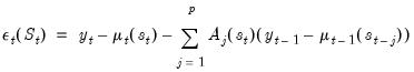 | (49.7) |
where
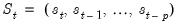
is a

dimensional state vector representing the current and

previous regimes, with

.
To simplify notation, in switching mean specifications

should be interpreted as shorthand for

being equal to the

-th possible realization of the

dimensional vector, as in
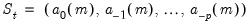 | (49.8) |
where

is the value of the

-th lagged state in the

-th possible realization, for
.
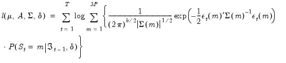
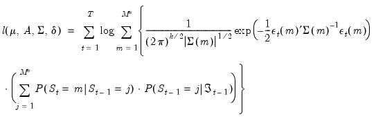
Log Likelihood
The likelihood contribution for a given observation may be formed by weighting the state specific multivariate normal density
Equation (49.4) by the one-step ahead prediction of the probability of being in the given state:
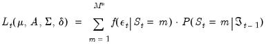 | (49.9) |
where
is obtained from the regime specific specifications
Equation (49.6) and
Equation (49.7).
,
,
, are the VAR parameters,

are parameters that determine the regime probabilities.
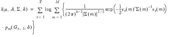
Defining

, we have the full normal mixture log-likelihood
 | (49.10) |
which may be maximized with respect to

.
It is worth noting that the likelihood function for this normal mixture model is unbounded for certain parameter values. However, local optima have the usual consistency, asymptotic normality, and efficiency properties. See Maddala (1986) for discussion of this issue as well as a survey of different algorithms and approaches for estimating the parameters.
Given parameter point-estimates, coefficient covariances may be estimated using conventional methods, e.g., inverse negative Hessian, inverse outer-product of the scores, and robust sandwich.
Regime Probabilities
To finish our likelihood specification, we must specify the regime probabilities function
There are two commonly employed forms: simple switching and Markov switching.
Simple Switching
The simple switching model features independent regime probabilities which do not depend on past states.
 | (49.11) |
More generally, we may allow for varying probabilities by assuming that

is a function of vectors of exogenous observables

and coefficients

parameterized using a multinomial logit specification:
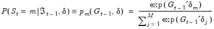 | (49.12) |
for
with the identifying normalization

. The special case of constant probabilities is handled by choosing

to be identically equal to 1.
Markov Switching
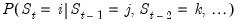
The first-order Markov assumption requires that the probability of being in a regime depends only on the previous state, so that
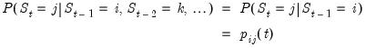 | (49.13) |
Typically, these transition probabilities are assumed to be time-invariant so that

for all

, but this restriction is not required.
We may write these probabilities in a transition matrix
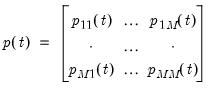 | (49.14) |
where the

-th element represents the probability of transitioning from regime

in period

to regime

in period

. (Note that some authors use the transpose of

so that all of their indices are reversed from those used here.)
As in the simple switching model, we may parameterize the probabilities in terms of a multinomial logit. Note that since each row of the transition matrix specifies a full set of conditional probabilities, we define a separate multinomial specification for each row

of the matrix
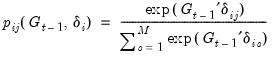 | (49.15) |
for

and

with the normalizations

.
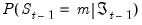
Probability Prediction and Filtering
The likelihood function in
Equation (49.10) depends on the one-step ahead predicted probabilities of being in a regime:
. Obtaining these predicted probabilities is central to the evaluation of the likelihood.
Of related interest are the contemporaneous estimates of the regime probabilities:
. The observed value of the dependent variable provides information about which regime is in effect in a given period, and we may use this contemporaneous information to updated our estimates of the regime probabilities. The process by which the predicted

probability estimates are updated to form

is commonly termed
filtering.
In the following sections, we outline the basics of one-step ahead prediction and filtering for both the simple switching specification and Markov switching.
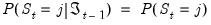
Simple Switching
One-step ahead prediction is straightforward for simple switching since the one-step ahead predicted probabilities are simply the specified probability functions:
In the switching intercept case, substituting the general form of the simple switching function
Equation (49.12) into
Equation (49.10), we get
 | (49.16) |
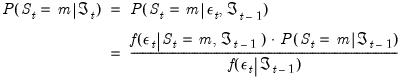
By Bayes’ theorem and the laws of conditional probability, we have the filtering expressions:
Substituting, we obtain the filtering update
 | (49.17) |
Note that in the switching model setting, the state variable is

-dimensional, so the above relationship does not apply. We must instead treat this model as a restricted form of the Markov switching model (as described below) where there no state dependence in the probability function.
Markov Switching
The Markov property of the transition probabilities implies that the expressions on the right-hand side of
Equation (49.10) must be evaluated recursively.
Briefly, each recursion step begins with filtered estimates of the regime probabilities for the previous period. Given filtered probabilities,
, the recursion may broken down into three steps:
1. We first form the one-step ahead predictions of the regime probabilities using basic rules of probability and the Markov transition matrix:
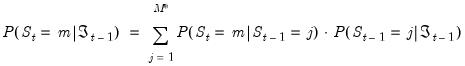 | (49.18) |
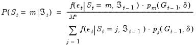
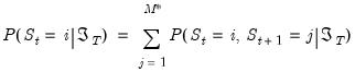
2. Next, we use these one-step ahead probabilities to form the one-step ahead joint densities of the data and regimes in period

:
 | (49.19) |
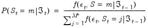
3. The likelihood contribution for period

is obtained by summing the joint probabilities across unobserved states to obtain the marginal distribution of the observed data
 | (49.20) |
4. The final step is to filter the probabilities by using the results in
Equation (49.19) to update one-step ahead predictions of the probabilities:
 | (49.21) |
These steps are repeated successively for each period,

. All that we require for implementation are the initial filtered probabilities,
, or alternately, the initial one-step ahead regime probabilities
. See
“Initial Probabilities” for discussion.
The likelihood obtained by summing the terms in
Equation (49.20) yields
 | (49.22) |
The likelihood may be maximized with respect to the parameters

using iterative methods. Coefficient covariances may be estimated using standard approaches.
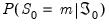
Initial Probabilities
In the switching intercept form, the Markov switching filter requires initialization of the filtered regime probabilities in period 0,
.
There are a few ways to proceed. Most commonly, the initial regime probabilities are set to the ergodic (steady state) values implied by the Markov transition matrix (see, for example Hamilton (1999, p. 192) or Kim and Nelson (1999, p. 70) for discussion and results). The values are thus treated as functions of the parameters that determine the transition matrix.
Alternately, we may use prior knowledge to specify regime probability values, or we can be agnostic and assign equal probabilities to regimes. Lastly, we may treat the initial probabilities as parameters to be estimated.
Note that the initialization to ergodic values using period 0 information is somewhat arbitrary in the case of time-varying transition probabilities.
In the switching means setting, the Markov switching filter requires initialization of the vector of probabilities associated with the

dimensional state vector. We may proceed as in the uncorrelated model by setting

initial probabilities in period

as described above, and recursively applying Markov transition updates to obtain the joint initial probabilities for the

dimensional initial probability vector in period

.
Again note that the initialization to steady state values using the period

information is somewhat arbitrary in the case of time-varying transition probabilities.
Smoothing
For the Markov switching specification, estimates of the regime probabilities may be improved by using all of the information in the sample. The
smoothed estimates for the regime probabilities in period

use the information set in the final period,

, in contrast to the filtered estimates which employ contemporaneous information,

.
Intuitively, using information about future realizations of the dependent variable

(

) improves our estimates of being in regime

in period

because the Markov transition probabilities link together the likelihood of the observed data in different periods.
Kim (2004) provides an efficient smoothing algorithm that requires only a single backward recursion through the data. Under the Markov assumption, Kim shows that the joint probability is given by
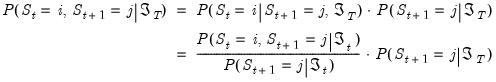 | (49.23) |
The key in moving from the first to the second line of
Equation (49.23) is the fact that under appropriate assumptions, if

were known, there is no additional information about

in the future data
.
The smoothed probability in period

is then obtained by marginalizing the joint probability with respect to

:
 | (49.24) |
Note that apart from the smoothed probability terms,
, all of the terms on the right-hand side of
Equation (49.23) are obtained as part of the filtering computations. Given the set of filtered probabilities, we initialize the smoother using
, and iterate computation of
Equation (49.23) and
Equation (49.24) for
to obtain the smoothed values.