How to Create and Specify a System
To estimate the parameters of your system of equations, you should first create a system object and specify the system of equations. There are three ways to specify the system: manually by entering a specification, by inserting a text file containing the specification, or by letting EViews create a system automatically from a selected list of variables,
To create a new system manually or by inserting a text file, click on or type system in the command window. A blank system object window should appear. You will fill the system specification window with text describing the equations, and potentially, lines describing the instruments and the parameter starting values. You may enter the text by typing in the specification, or clicking on the button and loading a specification from a text file. You may also insert a text file using the right-mouse button menu and selecting
To estimate the parameters of your system of equations, you should first create a system object and specify the system of equations. Click on or type system in the command window. The system object window should appear. When you first create the system, the window will be blank. You will fill the system specification window with text describing the equations, and potentially, lines describing the instruments and the parameter starting values.
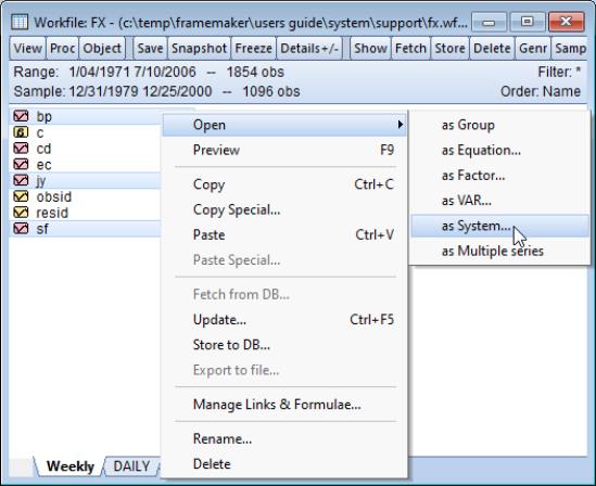
From a list of selected variables, EViews can also automatically generate linear equations in a system. To use this procedure, first highlight the dependent variables that will be in the system. Next, double click on any of the highlighted series, and select , or right click and select . The
Make System dialog box should appear with the variable names entered in the
Dependent variables field. You can augment the specification by adding regressors or AR terms, either estimated with common or equation specific coefficients. See
“System Procs” for additional details on this dialog.
The proc is also available from a Group object (see
“Make System”).
Equations
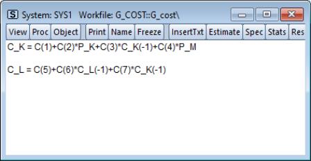
Enter your equations, by formula, using standard EViews expressions. The equations in your system should be behavioral equations with unknown coefficients and an implicit error term.
Consider the specification of a simple two equation system. You can use the default EViews coefficients, C(1), C(2), and so on, or you can use other coefficient vectors, in which case you should first declare them by clicking in the main menu.
There are some general rules for specifying your equations:
• Equations can be nonlinear in their variables, coefficients, or both. Cross equation coefficient restrictions may be imposed by using the same coefficients in different equations. For example:
y = c(1) + c(2)*x
z = c(3) + c(2)*z + (1-c(2))*x
• You may also impose adding up constraints. Suppose for the equation:
y = c(1)*x1 + c(2)*x2 + c(3)*x3
you wish to impose C(1)+C(2)+C(3)=1. You can impose this restriction by specifying the equation as:
y = c(1)*x1 + c(2)*x2 + (1-c(1)-c(2))*x3
• The equations in a system may contain autoregressive (AR) error specifications, but not MA, SAR, or SMA error specifications. You must associate coefficients with each AR specification. Enclose the entire AR specification in square brackets and follow each AR with an “=”-sign and a coefficient. For example:
cs = c(1) + c(2)*gdp + [ar(1)=c(3), ar(2)=c(4)]
You can constrain all of the equations in a system to have the same AR coefficient by giving all equations the same AR coefficient number, or you can estimate separate AR processes, by assigning each equation its own coefficient.
• Equations in a system need not have a dependent variable followed by an equal sign and then an expression. The “=”‑sign can be anywhere in the formula, as in:
log(unemp/(1-unemp)) = c(1) + c(2)*dmr
You can also write the equation as a simple expression without a dependent variable, as in:
(c(1)*x + c(2)*y + 4)^2
When encountering an expression that does not contain an equal sign, EViews sets the entire expression equal to the implicit error term.
If an equation should not have a disturbance, it is an identity, and should not be included in a system. If necessary, you should solve out for any identities to obtain the behavioral equations.
You should make certain that there is no identity linking all of the disturbances in your system. For example, if each of your equations describes a fraction of a total, the sum of the equations will always equal one, and the sum of the disturbances will identically equal zero. You will need to drop one of these equations to avoid numerical problems.
Instruments
If you plan to estimate your system using two-stage least squares, three-stage least squares, or GMM, you must specify the instrumental variables to be used in estimation. There are several ways to specify your instruments, with the appropriate form depending on whether you wish to have identical instruments in each equation, and whether you wish to compute the projections on an equation-by-equation basis, or whether you wish to compute a restricted projection using the stacked system.
In the simplest (default) case, EViews will form your instrumental variable projections on an equation-by-equation basis. If you prefer to think of this process as a two-step (2SLS) procedure, the first-stage regression of the variables in your model on the instruments will be run separately for each equation.
In this setting, there are two ways to specify your instruments. If you would like to use identical instruments in every equations, you should include a line beginning with the keyword “@INST” or “INST”, followed by a list of all the exogenous variables to be used as instruments. For example, the line:
@inst gdp(-1 to -4) x gov
instructs EViews to use these six variables as instruments for all of the equations in the system. System estimation will involve a separate projection for each equation in your system.
You may also specify different instruments for each equation by appending an “@”‑sign at the end of the equation, followed by a list of instruments for that equation. For example:
cs = c(1)+c(2)*gdp+c(3)*cs(-1) @ cs(-1) inv(-1) gov
inv = c(4)+c(5)*gdp+c(6)*gov @ gdp(-1) gov
The first equation uses CS(-1), INV(-1), GOV, and a constant as instruments, while the second equation uses GDP(-1), GOV, and a constant as instruments.
Lastly, you can mix the two methods. Any equation without individually specified instruments will use the instruments specified by the @inst statement. The system:
@inst gdp(-1 to -4) x gov
cs = c(1)+c(2)*gdp+c(3)*cs(-1)
inv = c(4)+c(5)*gdp+c(6)*gov @ gdp(-1) gov
will use the instruments GDP(-1), GDP(-2), GDP(-3), GDP(-4), X, GOV, and C, for the CS equation, but only GDP(-1), GOV, and C, for the INV equation.
As noted above, the EViews default behavior is to perform the instrumental variables projection on an equation-by-equation basis. You may, however, wish to perform the projections on the stacked system. Notably, where the number of instruments is large, relative to the number of observations, stacking the equations and instruments prior to performing the projection may be the only feasible way to compute 2SLS estimates.
To designate instruments for a stacked projection, you should use the @stackinst statement (note: this statement is only available for systems estimated by 2SLS or 3SLS; it is not available for systems estimated using GMM).
In a @stackinst statement, the “@STACKINST” keyword should be followed by a list of stacked instrument specifications. Each specification is a comma delimited list of series enclosed in parentheses (one per equation), describing the instruments to be constrained in a stacked specification.
For example, the following @stackinst specification creates two instruments in a three equation model:
@stackinst (z1,z2,z3) (m1,m1,m1)
This statement instructs EViews to form two stacked instruments, one by stacking the separate series Z1, Z2, and Z3, and the other formed by stacking M1 three times. The first-stage instrumental variables projection is then of the variables in the stacked system on the stacked instruments.
When working with systems that have a large number of equations, the above syntax may be unwieldy. For these cases, EViews provides a couple of shortcuts. First, for instruments that are identical in all equations, you may use an “*” after the comma to instruct EViews to repeat the specified series. Thus, the above statement is equivalent to:
@stackinst (z1,z2,z3) (m1,*)
Second, for non-identical instruments, you may specify a set of stacked instruments using an EViews group object, so long as the number of variables in the group is equal to the number of equations in the system. Thus, if you create a group Z with,
group z z1 z2 z3
the above statement can be simplified to:
@stackinst z (m1,*)
You can, of course, combine ordinary instrument and stacked instrument specifications. This situation is equivalent to having common and equation specific coefficients for variables in your system. Simply think of the stacked instruments as representing common (coefficient) instruments, and ordinary instruments as representing equation specific (coefficient) instruments. For example, consider the system given by,
@stackinst (z1,z2,z3) (m1,*)
@inst ia
y1 = c(1)*x1
y2 = c(1)*x2
y3 = c(1)*x3 @ ic
The stacked instruments for this specification may be represented as:
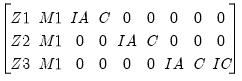 | (43.2) |
so it is easy to see that this specification is equivalent to the following stacked specification,
@stackinst (z1, z2, z3) (m1, *) (ia, 0, 0) (0, ia, 0) (0, 0, ia) (0, 0, ic)
since the common instrument specification,
@inst ia
is equivalent to:
@stackinst (ia, 0, 0) (0, ia, 0) (0, 0, ia)
Note that the constant instruments are added implicitly.
Additional Comments
• If you include a “C” in the stacked instrument list, it will not be included in the individual equations. If you do not include the “C” as a stacked instrument, it will be included as an instrument in every equation, whether specified explicitly or not.
• You should list all exogenous right-hand side variables as instruments for a given equation.
• Identification requires that there should be at least as many instruments (including the constant) in each equation as there are right-hand side variables in that equation.
• The @stackinst statement is only available for estimation by 2SLS and 3SLS. It is not currently supported for GMM.
• If you estimate your system using a method that does not use instruments, all instrument specification lines will be ignored.
Starting Values
For systems that contain nonlinear equations, you can include a line that begins with param to provide starting values for some or all of the parameters. List pairs of parameters and values. For example:
param c(1) .15 b(3) .5
sets the initial values of C(1) and B(3). If you do not provide starting values, EViews uses the values in the current coefficient vector. In ARCH estimation, by default, EViews does provide a set of starting coefficients. Users are able to provide their own set of starting values by selecting User Supplied in the Starting coefficient value field located in the Options tab.
How to Estimate a System
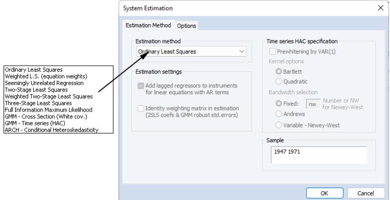
Once you have created and specified your system, you may push the Estimate button on the toolbar to bring up the System Estimation dialog.
The drop-down menu marked Estimation provides you with several options for the estimation method. You may choose from one of a number of methods for estimating the parameters of your specification.
The estimation dialog may change to reflect your choice, providing you with additional options. If you select an estimator which uses instrumental variables, a checkbox will appear, prompting you to choose whether to . As the checkbox label suggests, if selected, EViews will add lagged values of the dependent and independent variable to the instrument list when estimating AR models. The lag order for these instruments will match the AR order of the specification. This automatic lag inclusion reflects the fact that EViews transforms the linear specification to a nonlinear specification when estimating AR models, and that the lagged values are ideal instruments for the transformed specification. If you wish to maintain precise control over the instruments added to your model, you should unselect this option.
GMM Settings
Additional options appear if you are estimating a GMM specification. Note that the GMM-Cross section option uses a weighting matrix that is robust to heteroskedasticity and contemporaneous correlation of unknown form, while the GMM-Time series (HAC) option extends this robustness to autocorrelation of unknown form.
If you select either GMM method, EViews will display a checkbox labeled . If selected, EViews will estimate the model using identity weights, and will use the estimated coefficients and GMM specification you provide to compute a coefficient covariance matrix that is robust to cross-section heteroskedasticity (White) or heteroskedasticity and autocorrelation (Newey-West). If this option is not selected, EViews will use the GMM weights both in estimation, and in computing the coefficient covariances.
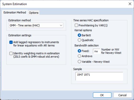
When you select the
GMM-Time series (HAC) option, the dialog displays additional options for specifying the weighting matrix. The new options will appear on the right side of the dialog. These options control the computation of the heteroskedasticity and autocorrelation robust (HAC) weighting matrix. See
“Technical Discussion” for a more detailed discussion of these options.
The Kernel Options determines the functional form of the kernel used to weight the autocovariances to compute the weighting matrix. The Bandwidth Selection option determines how the weights given by the kernel change with the lags of the autocovariances in the computation of the weighting matrix. If you select Fixed bandwidth, you may enter a number for the bandwidth or type nw to use Newey and West’s fixed bandwidth selection criterion.
The Prewhitening option runs a preliminary VAR(1) prior to estimation to “soak up” the correlation in the moment conditions.
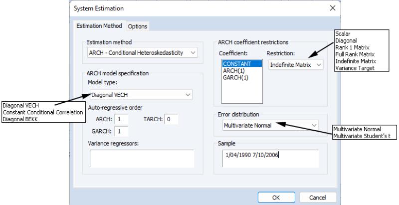
ARCH Settings
If the ARCH - Conditional Heteroskedasticity method is selected, the dialog displays the options appropriate for ARCH models. Model type allows you to select among three different multivariate ARCH models: Diagonal VECH, Constant Conditional Correlation (CCC), and Diagonal BEKK. Auto-regressive order indicates the number of autoregressive terms included in the model. You may use the Variance Regressors edit field to specify any regressors in the variance equation.
The coefficient specifications for the auto-regressive terms and regressors in the variance equation may be fine-tuned using the controls in the ARCH coefficient restrictions section of the dialog page. Each auto-regression or regressor term is displayed in the Coefficient list. You should select a term to modify it, and in the Restriction field select a type coefficient specification for that term. For the Diagonal VECH model, each of the coefficient matrices may be restricted to be Scalar, Diagonal, Rank One, Full Rank, Indefinite Matrix or (in the case of the constant coefficient) Variance Target. The options for the BEKK model behave the same except that the ARCH, GARCH, and TARCH term is restricted to be . For the CCC model, is the only option for ARCH, TARCH and GARCH terms, and are allowed or the constant term. For for exogenous variables you may choose between Individual and Common, indicating whether the parameters are restricted to be the same for all variance equations (common) or are unrestricted.
By default, the conditional distribution of the error terms is assumed to be Multivariate Normal. You have the option of instead using by selecting it in the Error distribution dropdown list.
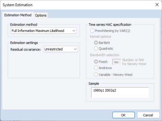
FIML Settings
For systems estimated using FIML, you will be prompted to specify estimation settings for the parameterization of the residual covariance matrix.
The drop down allows you to choose between the default , and , , and settings.
• The setting specifies standard FIML estimation in which all of the elements of the residual covariance matrix are estimated along with the coefficients of the mean equation. Note that the variance parameters for FIML are treated as nuisance parameters.
• The setting places zero restrictions on the off-diagonals of the residual covariance matrix. Only the diagonal elements of the residual covariance matrix corresponding to the variances are estimated.
• allows you to provide the name of a sym matrix object containing values for all of the residual covariances. All elements of the residual covariance

must be specified; no elements will be estimated.
• offers an alternative method of specifying the residual covariance. Instead of providing a sym matrix containing values of

, you will provide the name of a matrix

where

. Again, no elements of the residual covariance matrix are estimated.
Note that system objects estimated using a restricted FIML (diagonal, user-specified, or user-factor) estimator are not backward compatible with earlier versions of EViews, and will be dropped from the workfile if opened in a version prior to 9.5.
Options
For weighted least squares, SUR, weighted TSLS, 3SLS, GMM, and nonlinear systems of equations, there are additional options controlling the procedure for computing the GLS weighting matrix and the coefficient vector and for ARCH system, the coefficient vector used in estimation, as well as backcasting and robust standard error options.
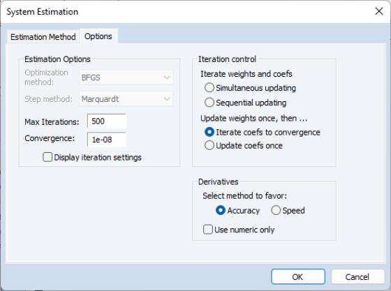
To specify the method used in iteration, click on the s tab.
The estimation option controls the method of iterating over coefficients, over the weighting matrices, or both:
• Update weights once, then—Iterate coefs to convergence is the default method.
By default, EViews carries out a first-stage estimation of the coefficients using no weighting matrix (the identity matrix). Using starting values obtained from OLS (or TSLS, if there are instruments), EViews iterates the first-stage estimates until the coefficients converge. If the specification is linear, this procedure involves a single OLS or TSLS regression.
The residuals from this first-stage iteration are used to form a consistent estimate of the weighting matrix.
In the second stage of the procedure, EViews uses the estimated weighting matrix in forming new estimates of the coefficients. If the model is nonlinear, EViews iterates the coefficient estimates until convergence.
• Update weights once, then—Update coefs once performs the first-stage estimation of the coefficients, and constructs an estimate of the weighting matrix. In the second stage, EViews does not iterate the coefficients to convergence, instead performing a single coefficient iteration step. Since the first stage coefficients are consistent, this one-step update is asymptotically efficient, but unless the specification is linear, does not produce results that are identical to the first method.
• Iterate Weights and Coefs—Simultaneous updating updates both the coefficients and the weighting matrix at each iteration. These steps are then repeated until both the coefficients and weighting matrix converge. This is the iteration method employed in EViews prior to version 4.
• Iterate Weights and Coefs—Sequential updating repeats the default method of updating weights and then iterating coefficients to convergence until both the coefficients and the weighting matrix converge.
Note that all four of the estimation techniques yield results that are asymptotically efficient. For linear models, the two Iterate Weights and Coefs options are equivalent, and the two One-Step Weighting Matrix options are equivalent, since obtaining coefficient estimates does not require iteration.
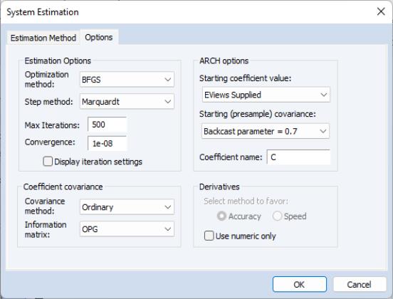
When ARCH is the estimation method a set of ARCH options appears:
• Starting coefficient value indicates what starting values EViews should use to start the iteration process. By default EViews Supplied is set. You can also select User Supplied which allows you to set your own starting coefficient via the C coefficient vector or another of your choice.
• Coefficient name specifies the name of the coefficient to be used in the variance equation. This can be different from the mean equation.
• Starting (presample) covariance indicates the method by which presample conditional variance and expected innovation should be calculated. Initial variance for the conditional variance are set using backcasting of the innovations,
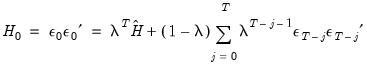 | (43.3) |
where:
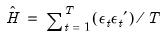 | (43.4) |
is the unconditional variance of the residuals. By default, the smoothing parameter,

is set to 0.7. However, you have the option to choose from a number of weights from 0.1 to 1, in increments of 0.1. Notice that if the parameter is set to 1 the initial value is simply the unconditional variance,
i.e. backcasting is not performed.
• EViews will report the robust standard errors when the Bollerslev-Wooldridge SE box is checked.
For basic specifications, ARCH analytic derivatives are available, and are employed by default. For a more complex model, either in the means or conditional variance, numerical or a combination of numerical and analytics are used. Analytic derivatives are generally, but not always, faster than numeric.
In addition, the
Options tab allows you to set a number of options for estimation, including convergence criterion, maximum number of iterations, and derivative calculation settings. See
“Setting Estimation Options” for related discussion.
Estimation Output
The system estimation output contains parameter estimates, standard errors, and t-statistics (or z-statistics for maximum likelihood estimations), for each of the coefficients in the system. Additionally, EViews reports the determinant of the residual covariance matrix, and, for ARCH and FIML estimates, the maximized likelihood values, Akaike and Schwarz criteria. For ARCH estimations, the mean equation coefficients are separated from the variance coefficient section.
In addition, EViews reports a set of summary statistics for each equation. The

statistic, Durbin-Watson statistic, standard error of the regression, sum-of-squared residuals, etc., are computed for each equation using the standard definitions, based on the residuals from the system estimation procedure.
In ARCH estimations, the raw coefficients of the variance equation do not necessarily give a clear understanding of the variance equations in many specifications. An extended coefficient view is supplied at the end of the output table to provide an enhanced view of the coefficient values involved.
You may access most of these results using regression statistics functions. See
(here) for a discussion of the use of these functions, and
“Object View and Procedure Reference” for a full listing of the available functions for systems.