Stability Diagnostics
EViews provides several test statistic views that examine whether the parameters of your model are stable across various subsamples of your data.
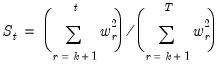
One common approach is to split the

observations in your data set of observations into

observations to be used for estimation, and
observations to be used for testing and evaluation. In time series work, you will usually take the first

observations for estimation and the last

for testing. With cross-section data, you may wish to order the data by some variable, such as household income, sales of a firm, or other indicator variables and use a subset for testing.
Note that the alternative of using all available sample observations for estimation promotes a search for a specification that best fits that specific data set, but does not allow for testing predictions of the model against data that have not been used in estimating the model. Nor does it allow one to test for parameter constancy, stability and robustness of the estimated relationship.
There are no hard and fast rules for determining the relative sizes of

and

. In some cases there may be obvious points at which a break in structure might have taken place—a war, a piece of legislation, a switch from fixed to floating exchange rates, or an oil shock. Where there is no reason
a priori to expect a structural break, a commonly used rule-of-thumb is to use 85 to 90 percent of the observations for estimation and the remainder for testing.
EViews provides built-in procedures which facilitate variations on this type of analysis.
Chow's Breakpoint Test
The idea of the breakpoint Chow test is to fit the equation separately for each subsample and to see whether there are significant differences in the estimated equations. A significant difference indicates a structural change in the relationship. For example, you can use this test to examine whether the demand function for energy was the same before and after the oil shock. The test may be used with least squares and two-stage least squares regressions; equations estimated using GMM offer a related test (see
“GMM Breakpoint Test”).
By default the Chow breakpoint test tests whether there is a structural change in all of the equation parameters. However if the equation is linear EViews allows you to test whether there has been a structural change in a subset of the parameters.
To carry out the test, we partition the data into two or more subsamples. Each subsample must contain more observations than the number of coefficients in the equation so that the equation can be estimated. The Chow breakpoint test compares the sum of squared residuals obtained by fitting a single equation to the entire sample with the sum of squared residuals obtained when separate equations are fit to each subsample of the data.
EViews reports three test statistics for the Chow breakpoint test. The F-statistic is based on the comparison of the restricted and unrestricted sum of squared residuals and in the simplest case involving a single breakpoint, is computed as:
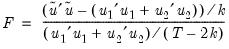 | (26.25) |
where

is the restricted sum of squared residuals,

is the sum of squared residuals from subsample

,

is the total number of observations, and

is the number of parameters in the equation. This formula can be generalized naturally to more than one breakpoint. The
F-statistic has an exact finite sample
F-distribution if the errors are independent and identically distributed normal random variables.
The log likelihood ratio statistic is based on the comparison of the restricted and unrestricted maximum of the (Gaussian) log likelihood function. The LR test statistic has an asymptotic

distribution with degrees of freedom equal to

under the null hypothesis of no structural change, where

is the number of subsamples.
The Wald statistic is computed from a standard Wald test of the restriction that the coefficients on the equation parameters are the same in all subsamples. As with the log likelihood ratio statistic, the Wald statistic has an asymptotic

distribution with

degrees of freedom, where

is the number of subsamples.
One major drawback of the breakpoint test is that each subsample requires at least as many observations as the number of estimated parameters. This may be a problem if, for example, you want to test for structural change between wartime and peacetime where there are only a few observations in the wartime sample. The Chow forecast test, discussed below, should be used in such cases.
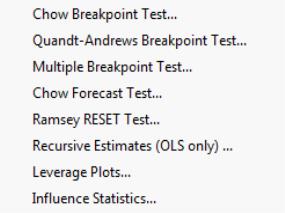
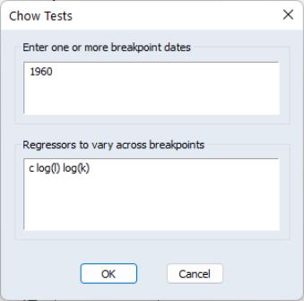
To apply the Chow breakpoint test, push on the equation toolbar. In the dialog that appears, list the dates or observation numbers for the breakpoints in the upper edit field, and the regressors that are allowed to vary across breakpoints in the lower edit field.
For example, if your original equation was estimated from 1950 to 1994, entering:
1960
in the dialog specifies two subsamples, one from 1950 to 1959 and one from 1960 to 1994. Typing:
1960 1970
specifies three subsamples, 1950 to 1959, 1960 to 1969, and 1970 to 1994.
The results of a test applied to EQ1 in the workfile “Coef_test.WF1”, using the settings above are:
Indicating that the coefficients are not stable across regimes.
Quandt-Andrews Breakpoint Test
The Quandt-Andrews Breakpoint Test tests for one or more unknown structural breakpoints in the sample for a specified equation. The idea behind the Quandt-Andrews test is that a single Chow Breakpoint Test is performed at every observation between two dates, or observations,

and

. The

test statistics from those Chow tests are then summarized into one test statistic for a test against the null hypothesis of no breakpoints between

and

.
By default the test tests whether there is a structural change in all of the original equation parameters. For linear specifications, EViews also allows you to test whether there has been a structural change in a subset of the parameters.
From each individual Chow Breakpoint Test two statistics are retained, the Likelihood Ratio
F-statistic and the Wald
F-statistic. The Likelihood Ratio
F-statistic is based on the comparison of the restricted and unrestricted sums of squared residuals. The Wald
F-statistic is computed from a standard Wald test of the restriction that the coefficients on the equation parameters are the same in all subsamples. Note that in linear equations these two statistics will be identical. For more details on these statistics, see
“Chow's Breakpoint Test”.
The individual test statistics can be summarized into three different statistics; the Sup or Maximum statistic, the Exp Statistic, and the Ave statistic (see Andrews, 1993 and Andrews and Ploberger, 1994). The Maximum statistic is simply the maximum of the individual Chow F-statistics:
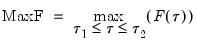 | (26.26) |
The Exp statistic takes the form:
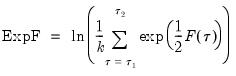 | (26.27) |
The Ave statistic is the simple average of the individual F-statistics:
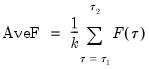 | (26.28) |
The distribution of these test statistics is non-standard. Andrews (1993) developed their true distribution, and Hansen (1997) provided approximate asymptotic
p-values. EViews reports the Hansen
p-values. The distribution of these statistics becomes degenerate as

approaches the beginning of the equation sample, or

approaches the end of the equation sample. To compensate for this behavior, it is generally suggested that the ends of the equation sample not be included in the testing procedure. A standard level for this “trimming” is 15%, where we exclude the first and last 15% of the observations. EViews sets trimming at 15% by default, but also allows the user to choose other levels. Note EViews only allows symmetric trimming,
i.e. the same number of observations are removed from the beginning of the estimation sample as from the end.
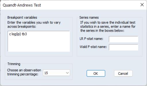
The Quandt-Andrews Breakpoint Test can be evaluated for an equation by selecting from the equation toolbar. The resulting dialog allows you to choose the level of symmetric observation trimming for the test, and, if your original equation was linear, which variables you wish to test for the unknown break point. You may also choose to save the individual Chow Breakpoint test statistics into new series within your workfile by entering a name for the new series.
As an example we estimate a consumption function, EQ02 in the workfile “DEMO.WF1”, using quarterly data from 1952Q1 to 1992Q4. To test for an unknown structural break point amongst all the original regressors we run the Quandt-Andrews test with 15% trimming. This test gives the following results:
Note all three of the summary statistic measures fail to reject the null hypothesis of no structural breaks at the 1% level within the 113 possible dates tested. The maximum statistic was in 1982Q2, and that is the most likely breakpoint location. Also, since the original equation was linear, note that the p-value for the LR F-statistic is identical to the Wald F-statistic.
Multiple Breakpoint Tests
Tests for parameter instability and structural change in regression models have been an important part of applied econometric work dating back to Chow (1960), who tested for regime change at
a priori known dates using an
F-statistic. To relax the requirement that the candidate breakdate be known, Quandt (1960) modified the Chow framework to consider the
F-statistic with the largest value over all possible breakdates. Andrews (1993) and Andrews and Ploberger (1994) derived the limiting distribution of the Quandt and related test statistics. The EViews tools for performing these tests are described in
“Chow's Breakpoint Test” and
“Quandt-Andrews Breakpoint Test”.
More recently, Bai (1997) and Bai and Perron (1998, 2003a) provide theoretical and computational results that further extend the Quandt-Andrews framework by allowing for multiple unknown breakpoints. The remainder of this section offers a brief outline of the Bai and Bai-Perron approach to structural break testing as implemented in EViews. Perron (2006) offers a useful survey of the literature and provides references for those requiring additional discussion.
Background
We consider a standard multiple linear regression model with

periods and

potential breaks (producing

regimes). For the observations
in regime

we have the regression model
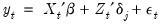 | (26.29) |
for the regimes

. Note that the regressors are divided into two groups. The

variables are those whose parameters do not vary across regimes, while the

variables have coefficients that are regime specific.
While it is slightly more convenient to define breakdates to be the last date of a regime, we follow EViews’s convention in defining the breakdate to be the first date of the subsequent regime. We tie down the endpoints by setting

and
.
The multiple breakpoint tests that we consider may broadly be divided into three categories: tests that employ global maximizers for the breakpoints, test that employ sequentially determined breakpoints, and hybrid tests, which combine the two approaches.
Global Maximizer Tests
Bai and Perron (1998) describe global optimization procedures for identifying the

multiple breaks which minimize the sums-of-squared residuals of the regression model
Equation (26.29).
Briefly, for a
specific set of

breakpoints, say
, we may minimize the sum-of-squared residuals:
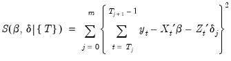 | (26.30) |
using standard least squares regression to obtain estimates

. The global

-break optimizers are the set of breakpoints and corresponding coefficient estimates that minimize sum-of-squares across
all possible sets of

-break partitions.
Note that the number of comparison models increases rapidly in both

and

so that efficient algorithms for computing the optimizers are required. Practical algorithms for computing the global optimizers for multiple breakpoint models are outlined in Bai and Perron (2003a).
These global breakpoint estimates are then used as the basis for several breakpoint tests. EViews supports both the Bai and Perron (1998) tests of

-breaks versus none test (along with the double maximum variants of this test in which

is determined as part of the testing procedure), and information criterion methods (Yao, 1988 and Liu, Wi, and Zidek, 1997) for determining the number of breaks.
Global L Breaks vs. None
Bai and Perron (1998) describe a generalization of the Quandt-Andrews test (Andrews, 1993) in which we test for equality of the

across multiple regimes. For a test of the null of no breaks against an alternative of

breaks, we employ an
F-statistic to evaluate the null hypothesis that
. The general form of the statistic (Bai-Perron 2003a) is:
 | (26.31) |
where

is the optimal

-break estimate of

,
, and

is an estimate of the variance covariance matrix of

which may be robust to serial correlation and heteroskedasticity, whose form depends on assumptions about the distribution of the data and the errors across segments. (We do not reproduce the formulae for the estimators of the variance matrices here as there are a large number of cases to consider; Bai-Perron (2003a) offer detailed descriptions of the various cases.)
A single test of no breaks against an alternative of

breaks assumes that the alternative number of breakpoints

is pre-specified. In cases where

is not known, we may test the null of no structural change against an unknown number of breaks up to some upper-bound,

. This type of testing is termed
double maximum since it involves maximization both for a given

and across various values of the test statistic for

.
The equal-weighted version of the test, termed

chooses the alternative that maximizes the statistic across the number of breakpoints. An alternative approach, denoted

applies weights to the individual statistics so that the implied marginal

-values are equal prior to taking the maximum.
The distributions of these test statistics are non-standard, but Bai and Perron (2003b) provide critical value and response surface computations for various trimming parameters (minimum sample sizes for estimating a break), numbers of regressors, and numbers of breaks.
Information Criteria
Yao (1988) shows that under relatively strong conditions, the number of breaks

that minimizes the Schwarz criterion is a consistent estimator of the true number of breaks in a breaking mean model.
More generally, Liu, Wu, and Zidek (1997) propose use of modified Schwarz criterion for determining the number of breaks in a regression framework. LWZ offer theoretical results showing consistency of the estimated number of breakpoints, and provide simulation results to guide the choice of the modified penalty criterion.
Sequential Testing Procedures
Bai (1997) describes an intuitive approach for detecting more than one break. The procedure involves sequential application of breakpoint tests.
• Begin with the full sample and perform a test of parameter constancy with unknown break.
• If the test rejects the null hypothesis of constancy, determine the breakdate, divide the sample into two samples and perform single unknown breakpoint tests in each subsample. Each of these tests may be viewed as a test of the alternative of

versus the null hypothesis of

breaks. Add a breakpoint whenever a subsample null is rejected. (Alternately, one could test only the single subsample which shows the greatest improvement in the sum-of-squared residuals.)
• Repeat the procedure until all of the subsamples do not reject the null hypothesis, or until the maximum number of breakpoints allowed or maximum subsample intervals to test is reached.
If the number of breakpoints is pre-specified, we simply estimate the specified number of breakpoints using the one-at-a-time method.
Once the sequential breakpoints have been determined, Bai recommends a refinement procedure whereby breakpoints are re-estimated if they are obtained from a subsample containing more than one break. This procedure is required so that the breakpoint estimates have the same limiting distribution as those obtained from the global optimization procedure.
Note that EViews uses the (potentially robust)
F-statistic in
Equation (26.31) for the test in place of the difference in sums-of-squared residuals described in Bai (1997) and Bai and Perron (1998). Critical value and response surface computations are again provided by Bai and Perron (2003b).
Global Plus Sequential Testing
Bai and Perron (1998) describe a modified Bai (1997) approach in which, at each test step, the

breakpoints under the null are obtained by global minimization of the sum-of-squared residuals. We may therefore view this approach as an

versus

test procedure that combines the global and sequential testing approaches.
Each test begins with the set of

global optimizing breakpoints and performs a single test of parameter constancy using the subsample break that most reduces the-sum-of-squared residuals. Note that in this case, we only test for constancy in a single subsample.
Computing Multiple Breakpoint Tests in EViews
To use the EViews tools for testing for multiple breaks, you must use an equation that is specified by list and estimated by least squares. Note in particular that this latter restriction means that models with AR and MA terms are not eligible for multiple break testing.
From an estimated equation, bring up the multiple break testing dialog, by clicking on .
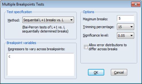
The dialog is divided into the , , and sections.
Test Specification
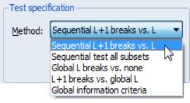
The section contains a drop-down where you may specify the type of test you wish to perform. You may choose between:
• Sequential L+1 breaks vs. L
• Sequential tests all subsets
• Global L breaks vs. none
• L+1 breaks vs. global L
• Global information criteria
The two sequential tests are based on the Bai sequential methodology as described in
“Sequential Testing Procedures” above. The methods differ in whether, for a given

breakpoints, we test for an additional breakpoint in each of the

segments (), or whether we test for the single added breakpoint that most reduces the sum-of-squares ().
The choice implements the Bai-Perron tests of

globally optimized breaks against the null of no structural breaks, along with the corresponding

and

tests (
“Global L Breaks vs. None”).
The choice implements the Bai-Perron

vs.

testing procedure outlined in
“Global Plus Sequential Testing”.
The uses the information criteria computed from the global optimizers to determine the number of breaks (
“Information Criteria”).
Breakpoint Variables
EViews supports the testing of partial structural change models in which only a subset of the variables in the regression are subject to change across regimes. The variables which have regime specific coefficients should be listed in the edit field.
By default, all of the variables in your specification will be included in this list. To treat some of these variables as non-varying

‘s, you may simply delete them from the list. Note that there must be at least one variable in the list.
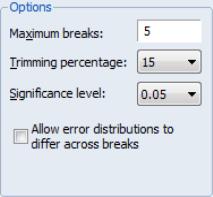
Options
The section of the dialog allow you to specify the maximum number of breaks or break levels to consider, the trimming percentage of the sample, the significance level for any test computations (if relevant), and assumptions regarding the computation of the variance matrices used in testing (if relevant):
• The limits the number of breakpoints allowed via global testing and in sequential or mixed

vs.

testing. If you have selected the method, the edit field will be labeled to indicate that the restriction is on the maximum number of break levels allowed. This change in labeling reflects the fact that the Bai all subsets approach potentially adds

breaks for a given set of

breaks.
• The
implicitly determines

, the minimum segment length permitted when constructing a test. Small values of the trimming percentage can lead to estimates of coefficients and variances which are based on very few observations.
In testing settings, you will be prompted to specify a test size, and to make assumptions about the distribution of the errors across segments which determine the form for the estimator

in
Equation (26.31).
• The drop-down menu should be used to choose between test size values of (0.01, 0.025, 0.05, and 0.10). This menu is not relevant for tests which select between models using information criteria.
• The lets you specify different error distributions for different regimes (which in turn implies using different estimators for

; see Bai and Perron, 2003b for details). Selecting this option will provide robustness of the test to error distribution variation at the cost of power if the error distributions are the same across regimes.
We remind you that EViews will employ the coefficient covariance settings in the original equation when determining whether to allow for heteroskedasticity alone or heteroskedasticity and serial correlation. Thus, if you estimated your original equation using White standard errors, EViews will compute the breakpoint tests using an statistic which is robust to heteroskedasticity. Similarly, if you estimated your original equation with Newey-West standard errors, EViews will compute the breakpoint tests using a HAC robust test statistic.
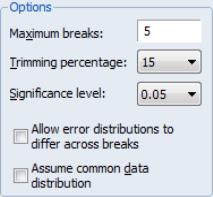
One final note. EViews will, by default, estimate the robust specification assuming heterogeneous distributions for the

. Bai and Perron (2003a) who, with one exception, do not impose the restriction that the distribution of the

is the same across regimes. In cases where you are testing using robust variances, EViews will offer you a choice of whether to assume a common distribution for the data across regimes.
Bai and Perron do impose the homogeneity data restriction when computing heteroskedasticity and HAC robust variances estimators assuming homogeneous errors. To match the Bai-Perron common error assumptions, you will have to select the .
(Note that EViews does not allow you to specify heterogeneous error distributions and robust covariances in partial switching models.)
Examples
To illustrate the use of these tools in practice, we consider a simple model of the U.S.
ex-post real interest rate from Garcia and Perron (1996) that is used as an example by Bai and Perron (2003a). The data, which consist of observations for the three-month treasury rate deflated by the CPI for the period 1961q1–1983q3, are provided in the series RATES in the workfile “realrate.WF1”. The regression model consists of a constant regressor, and allows for serial correlation that differs across regimes through the use of HAC covariance estimation. We allow up to 5 breaks in the model, and employ a trimming percentage of 15%

. Since there are 103 observations in the sample, the trimming value implies that regimes are restricted to have at least 15 observations.
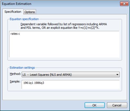
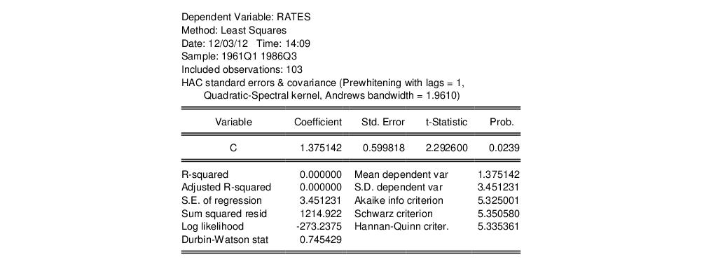
Following Bai and Perron (2003a), we begin by estimating the equation specification using least squares. Our equation specification consists of the dependent variable and a single (constant) regressor, so we enter
rate c
in the specification dialog
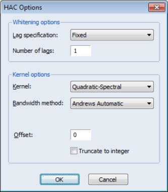
Since we wish to allow for serial correlation in the errors, we specify a quadratic spectral kernel based HAC covariance estimation using prewhitened residuals. The kernel bandwith is determined automatically using the Andrews AR(1) method.
The covariance options may be specified in the dialog by selecting the tab, clicking on the button and filling out the dialog as shown:
Click on to accept the HAC settings, and then on to estimate the equation. The estimation results should be as depicted below:
To construct multiple breakpoint tests for this equation, select from the equation dialog. We consider examples for three different approaches for multiple breakpoint testing with this equation.
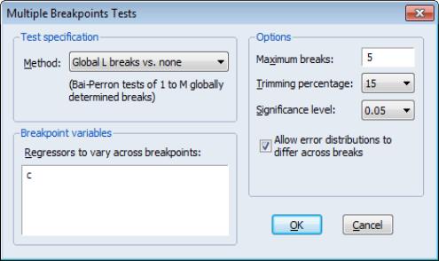
Sequential Bai-Perron
The default setting () instructs EViews to perform sequential testing of

versus

breaks using the methods outlined by Bai (1997) and Bai and Perron (1998).
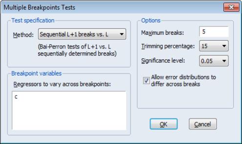
There is a single regressor “C” which we require to be in the list of breaking variables.
By default, the tests allow for a maximum number of 5 breaks, employ a trimming percentage of 15%, and use the 0.05 significance level for the sequential testing. We will leave these options at their default settings. We do, however, select the checkbox to allow for error heterogeneity.
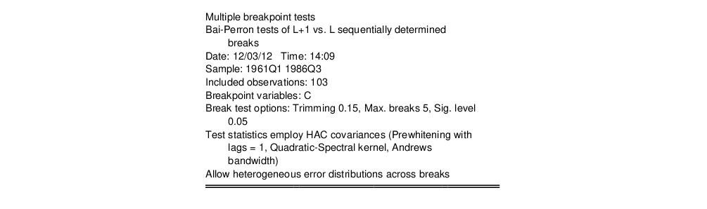
Click on to accept the test specification and display the test results. The top portion of the dialog shows the test settings, including the test method, breakpoint variables, test options, and method of computing test covariances. Note that the test employs the same HAC covariance settings used in the original equation but assume regime specific error distributions:
The middle section of the table presents the actual sequential test results:
EViews displays the F-statistic, along with the F-statistic scaled by the number of varying regressors (which is the same in this case, since we only have the single, varying regressor), and the Bai-Perron critical value for the scaled statistic. The sequential test results indicate that there are three breakpoints: we reject the nulls of 0, 1, and 2 breakpoints in favor of the alternatives of 1, 2, and 3 breakpoints, but the test of 4 versus 3 breakpoints does not reject the null.
The bottom portion of the output shows the estimated breakdates:
EViews displays both the breakdates obtained from the original sequential procedure, and those obtained following the repartition procedure. In this case, the dates do not change. Again bear in mind that the results follow the EViews convention in defining breakdates to be the first date of the subsequent regime.
Global Bai-Perron L Breaks vs. None
To perform the Bai-Perron tests of

globally optimized breaks against the null of no structural breaks, along with the corresponding

and

tests, simply call up the dialog and change the drop-down to :
We again leave the remaining settings at their default values with the exception of the checkbox which is selected. Click on to perform the test.
The top portion of the output, which shows the test settings, is almost identical to the output for the previous example. The only difference is a line identifying the test method as being “Bai-Perron tests of 1 to M globally determined breaks.”
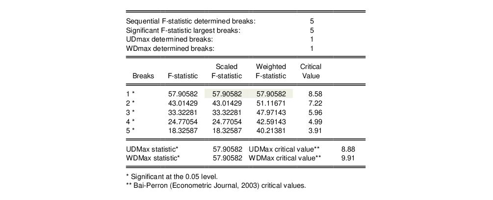
The middle portion of the output contains the test results:
The first four lines summarize the results for different approaches to determining the number of breaks. The “Sequential” result is obtained by performing tests from 1 to the maximum number until we cannot reject the null; the “Significant” result chooses the largest statistically significant breakpoint. In both cases, the multiple breakpoint test indicates that there are 5 breaks. The “UDmax” and “WDmax” results show the number of breakpoints as determined by application of the unweighted and weighted maximized statistics. The maximized statistics both indicate the presence of a single break.
The remaining lines show the individual test statistics (original, scaled, weighted) along with the critical values for the scaled statistics. In each case, the statistics far exceed the critical value so that we reject the null of no breaks. Note that the values corresponding to the

and

statistics are shaded for easy identification.
The last two lines of output show the test results for double maximum statistics. In both cases, the maximized value clearly exceeds the critical value, so that we reject the null of no breaks in favor of the alternative of a single break.
The bottom of the portion shows the global optimizers for the breakpoints for each number of breaks:
Note that the three-break global optimizers are the same as those obtained in the sequential testing example (
“Sequential Bai-Perron”). This equivalence will not hold in general.
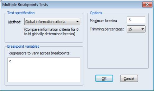
Global Information Criteria
Lastly, we consider using information criteria to select the number of breaks.
Here we see the dialog when we select in the drop-down menu. Note that there are no options for computing the coefficient covariances since this method does not require their calculation. Click on to construct the table of results.
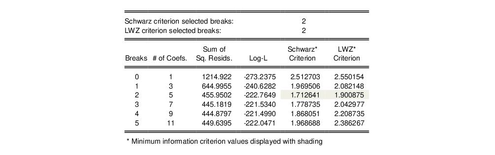
The top and bottom portions of the output are similar to the results seen previously so we focus only on the test summaries themselves:
The two summary rows show that both the Schwarz and the LWZ information criteria select 2 breaks. The remainder of the output shows, for each break, the number of estimated coefficients, the optimized sum-of-squared residuals and likelihood, and the values of the information criteria. The minimized Schwarz and LWZ values are shaded for easy identification.
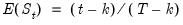
Chow's Forecast Test
The Chow forecast test estimates two models—one using the full set of data

, and the other using a long subperiod

. Differences between the results for the two estimated models casts doubt on the stability of the estimated relation over the sample period. The Chow forecast test can be used with least squares and two-stage least squares regressions.
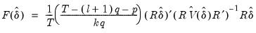
EViews reports two test statistics for the Chow forecast test. The F-statistic is computed as
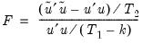 | (26.32) |
where

is the residual sum of squares when the equation is fitted to all

sample observations,

is the residual sum of squares when the equation is fitted to

observations, and

is the number of estimated coefficients. This
F-statistic follows an exact finite sample
F-distribution if the errors are independent, and identically, normally distributed.
The log likelihood ratio statistic is based on the comparison of the restricted and unrestricted maximum of the (Gaussian) log likelihood function. Both the restricted and unrestricted log likelihood are obtained by estimating the regression using the whole sample. The restricted regression uses the original set of regressors, while the unrestricted regression adds a dummy variable for each forecast point. The LR test statistic has an asymptotic

distribution with degrees of freedom equal to the number of forecast points

under the null hypothesis of no structural change.
To apply Chow’s forecast test, push on the equation toolbar and specify the date or observation number for the beginning of the forecasting sample. The date should be within the current sample of observations.
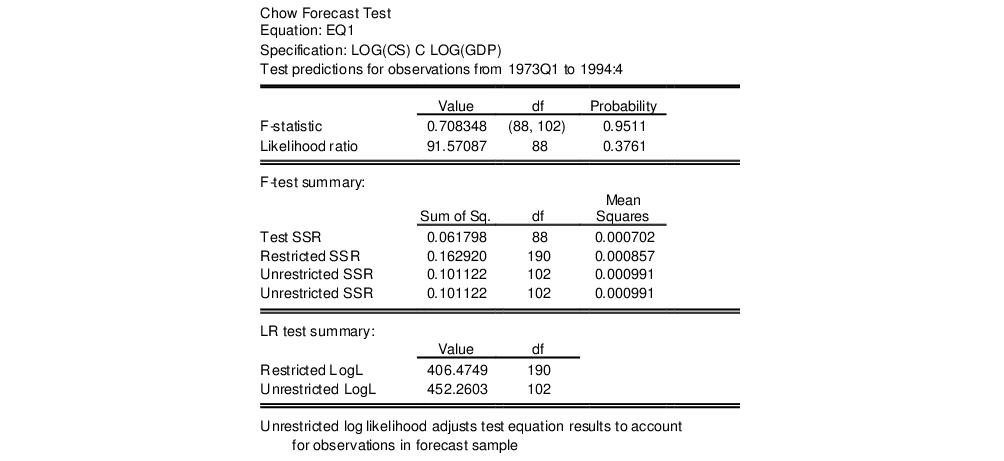
As an example, using the “Coef_test2.WF1” workfile, suppose we estimate a consumption function, EQ1, using quarterly data from 1947q1 to 1994q4 and specify 1973q1 as the first observation in the forecast period. The test reestimates the equation for the period 1947q1 to 1972q4, and uses the result to compute the prediction errors for the remaining quarters, and the top portion of the table shows the following results:
Neither of the forecast test statistics reject the null hypothesis of no structural change in the consumption function before and after 1973q1.
If we test the same hypothesis using the Chow breakpoint test, the result is:
Note that the breakpoint test statistics decisively reject the hypothesis from above. This example illustrates the possibility that the two Chow tests may yield conflicting results.
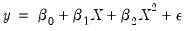
Ramsey's RESET Test
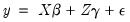
RESET stands for Regression Specification Error Test and was proposed by Ramsey (1969). The classical normal linear regression model is specified as:
 | (26.33) |
where the disturbance vector

is presumed to follow the multivariate normal distribution

. Specification error is an omnibus term which covers any departure from the assumptions of the maintained model. Serial correlation, heteroskedasticity, or non-normality of all violate the assumption that the disturbances are distributed

. Tests for these specification errors have been described above. In contrast, RESET is a general test for the following types of specification errors:
• Omitted variables;

does not include all relevant variables.
• Incorrect functional form; some or all of the variables in

and

should be transformed to logs, powers, reciprocals, or in some other way.
• Correlation between

and

, which may be caused, among other things, by measurement error in

, simultaneity, or the presence of lagged

values and serially correlated disturbances.
Under such specification errors, LS estimators will be biased and inconsistent, and conventional inference procedures will be invalidated. Ramsey (1969) showed that any or all of these specification errors produce a non-zero mean vector for

. Therefore, the null and alternative hypotheses of the RESET test are:
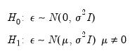 | (26.34) |
The test is based on an augmented regression:
 | (26.35) |
The test of specification error evaluates the restriction

. The crucial question in constructing the test is to determine what variables should enter the

matrix. Note that the

matrix may, for example, be comprised of variables that are not in the original specification, so that the test of

is simply the omitted variables test described above.
In testing for incorrect functional form, the nonlinear part of the regression model may be some function of the regressors included in

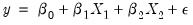
. For example, if a linear relation,
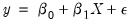 | (26.36) |
is specified instead of the true relation:
 | (26.37) |
the augmented model has

and we are back to the omitted variable case. A more general example might be the specification of an additive relation,
 | (26.38) |
instead of the (true) multiplicative relation:
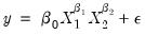 | (26.39) |
A Taylor series approximation of the multiplicative relation would yield an expression involving powers and cross-products of the explanatory variables. Ramsey's suggestion is to include powers of the predicted values of the dependent variable (which are, of course, linear combinations of powers and cross-product terms of the explanatory variables) in

:
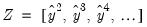 | (26.40) |
where

is the vector of fitted values from the regression of

on

. The superscripts indicate the powers to which these predictions are raised. The first power is not included since it is perfectly collinear with the

matrix.
Output from the test reports the test regression and the F-statistic and log likelihood ratio for testing the hypothesis that the coefficients on the powers of fitted values are all zero. A study by Ramsey and Alexander (1984) showed that the RESET test could detect specification error in an equation which was known a priori to be misspecified but which nonetheless gave satisfactory values for all the more traditional test criteria—goodness of fit, test for first order serial correlation, high t-ratios.
To apply the test, select and specify the number of fitted terms to include in the test regression. The fitted terms are the powers of the fitted values from the original regression, starting with the square or second power. For example, if you specify 1, then the test will add

in the regression, and if you specify 2, then the test will add

and

in the regression, and so on. If you specify a large number of fitted terms, EViews may report a near singular matrix error message since the powers of the fitted values are likely to be highly collinear. The Ramsey RESET test is only applicable to equations estimated using selected methods.
Recursive Least Squares
In recursive least squares the equation is estimated repeatedly, using ever larger subsets of the sample data. If there are

coefficients to be estimated in the

vector, then the first

observations are used to form the first estimate of

. The next observation is then added to the data set and

observations are used to compute the second estimate of

. This process is repeated until all the

sample points have been used, yielding

estimates of the

vector. At each step the last estimate of

can be used to predict the next value of the dependent variable. The one-step ahead forecast error resulting from this prediction, suitably scaled, is defined to be a
recursive residual.More formally, let

denote the

matrix of the regressors from period 1 to period

, and

the corresponding vector of observations on the dependent variable. These data up to period

give an estimated coefficient vector, denoted by

. This coefficient vector gives you a forecast of the dependent variable in period

. The forecast is

, where

is the row vector of observations on the regressors in period

. The forecast error is

, and the forecast variance is given by:
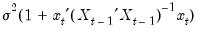 | (26.41) |
The recursive residual

is defined in EViews as:
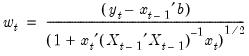 | (26.42) |
These residuals can be computed for
. If the maintained model is valid, the recursive residuals will be independently and normally distributed with zero mean and constant variance

.
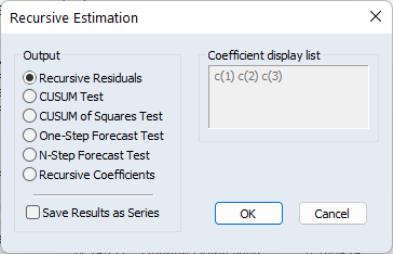
To calculate the recursive residuals, press on the equation toolbar. There are six options available for the recursive estimates view. The recursive estimates view is only available for equations estimated by ordinary least squares without AR and MA terms. The
Save Results as Series option allows you to save the recursive residuals and recursive coefficients as named series in the workfile; see
“Save Results as Series”.
Recursive Residuals
This option shows a plot of the recursive residuals about the zero line. Plus and minus two standard errors are also shown at each point. Residuals outside the standard error bands suggest instability in the parameters of the equation.
CUSUM Test
The CUSUM test (Brown, Durbin, and Evans, 1975) is based on the cumulative sum of the recursive residuals. This option plots the cumulative sum together with the 5% critical lines. The test finds parameter instability if the cumulative sum goes outside the area between the two critical lines.
The CUSUM test is based on the statistic:
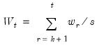 | (26.43) |
for

, where

is the recursive residual defined above, and
s is the standard deviation of the recursive residuals

. If the

vector remains constant from period to period,

, but if

changes,

will tend to diverge from the zero mean value line. The significance of any departure from the zero line is assessed by reference to a pair of 5% significance lines, the distance between which increases with

. The 5% significance lines are found by connecting the points:
 | (26.44) |
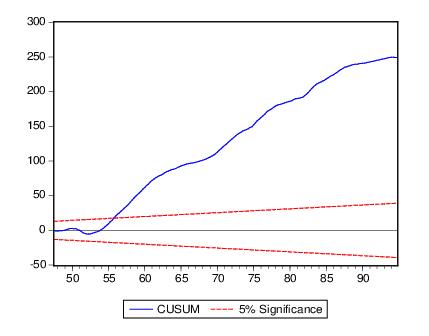
Movement of

outside the critical lines is suggestive of coefficient instability. A sample CUSUM is given below:
The test clearly indicates instability in the equation during the sample period.
CUSUM of Squares Test
The CUSUM of squares test (Brown, Durbin, and Evans, 1975) is based on the test statistic:
 | (26.45) |
The expected value of

under the hypothesis of parameter constancy is:
 | (26.46) |
which goes from zero at

to unity at

. The significance of the departure of

from its expected value is assessed by reference to a pair of parallel straight lines around the expected value. See Brown, Durbin, and Evans (1975) or Johnston and DiNardo (1997, Table D.8) for a table of significance lines for the CUSUM of squares test.
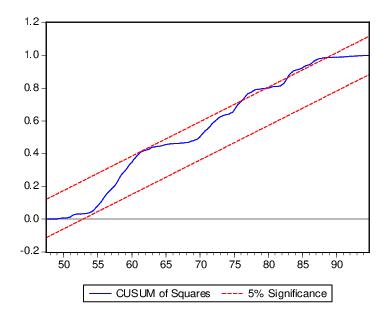
The CUSUM of squares test provides a plot of

against

and the pair of 5 percent critical lines. As with the CUSUM test, movement outside the critical lines is suggestive of parameter or variance instability.
The cumulative sum of squares is generally within the 5% significance lines, suggesting that the residual variance is somewhat stable.
One-Step Forecast Test
If you look back at the definition of the recursive residuals given above, you will see that each recursive residual is the error in a one-step ahead forecast. To test whether the value of the dependent variable at time

might have come from the model fitted to all the data up to that point, each error can be compared with its standard deviation from the full sample.
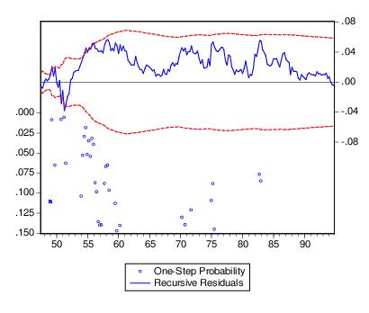
The One-Step Forecast Test option produces a plot of the recursive residuals and standard errors and the sample points whose probability value is at or below 15 percent. The plot can help you spot the periods when your equation is least successful. For example, the one-step ahead forecast test might look like this:
The upper portion of the plot (right vertical axis) repeats the recursive residuals and standard errors displayed by the Recursive Residuals option. The lower portion of the plot (left vertical axis) shows the probability values for those sample points where the hypothesis of parameter constancy would be rejected at the 5, 10, or 15 percent levels. The points with p-values less the 0.05 correspond to those points where the recursive residuals go outside the two standard error bounds.
For the test equation, there is evidence of instability early in the sample period.
N-Step Forecast Test
This test uses the recursive calculations to carry out a sequence of Chow Forecast tests. In contrast to the single Chow Forecast test described earlier, this test does not require the specification of a forecast period— it automatically computes all feasible cases, starting with the smallest possible sample size for estimating the forecasting equation and then adding one observation at a time. The plot from this test shows the recursive residuals at the top and significant probabilities (based on the F-statistic) in the lower portion of the diagram.
Recursive Coefficient Estimates
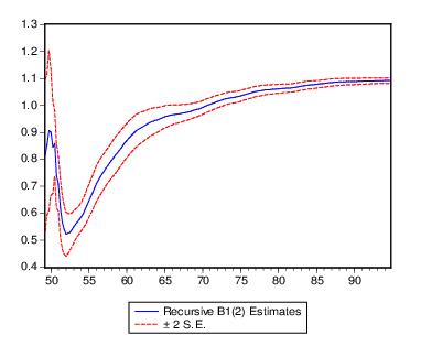
This view enables you to trace the evolution of estimates for any coefficient as more and more of the sample data are used in the estimation. The view will provide a plot of selected coefficients in the equation for all feasible recursive estimations. Also shown are the two standard error bands around the estimated coefficients.
If the coefficient displays significant variation as more data is added to the estimating equation, it is a strong indication of instability. Coefficient plots will sometimes show dramatic jumps as the postulated equation tries to digest a structural break.
To view the recursive coefficient estimates, click the Recursive Coefficients option and list the coefficients you want to plot in the Coefficient Display List field of the dialog box. The recursive estimates of the marginal propensity to consume (coefficient C(2)), from the sample consumption function are provided below:
The estimated propensity to consume rises steadily as we add more data over the sample period, approaching a value of one.
Save Results as Series
The Save Results as Series checkbox will do different things depending on the plot you have asked to be displayed. When paired with the Recursive Coefficients option, will instruct EViews to save all recursive coefficients and their standard errors in the workfile as named series. EViews will name the coefficients using the next available name of the form, R_C1, R_C2, …, and the corresponding standard errors as R_C1SE, R_C2SE, and so on.
If you check the Save Results as Series box with any of the other options, EViews saves the recursive residuals and the recursive standard errors as named series in the workfile. EViews will name the residual and standard errors as R_RES and R_RESSE, respectively.
Note that you can use the recursive residuals to reconstruct the CUSUM and CUSUM of squares series.
Leverage Plots
Leverage plots are the multivariate equivalent of a simple residual plot in a univariate regression. Like influence statistics, leverage plots can be used as a method for identifying influential observations or outliers, as well as a method of graphically diagnosing any potential failures of the underlying assumptions of a regression model.
Leverage plots are calculated by, in essence, turning a multivariate regression into a collection of univariate regressions. Following the notation given in Belsley, Kuh and Welsch 2004 (Section 2.1), the leverage plot for the k-th coefficient is computed as follows:
Let

be the
k-th column of the data matrix (the
k-th variable in a linear equation, or the
k-th gradient in a non-linear), and

be the remaining columns. Let

be the residuals from a regression of the dependent variable,

on

, and let

be the residuals from a regression of

on

. The leverage plot for the
k-th coefficient is then a scatter plot of

on

.
It can easily be shown that in an auxiliary regression of

on a constant and

, the coefficient on

will be identical to the
k-th coefficient from the original regression. Thus the original regression can be represented as a series of these univariate auxiliary regressions.
In a univariate regression, a plot of the residuals against the explanatory variable is often used to check for outliers (any observation whose residual is far from the regression line), or to check whether the model is possibly mis-specified (for example to check for linearity). Leverage plots can be used in the same way in a multivariate regression, since each coefficient has been modelled in a univariate auxiliary regression.
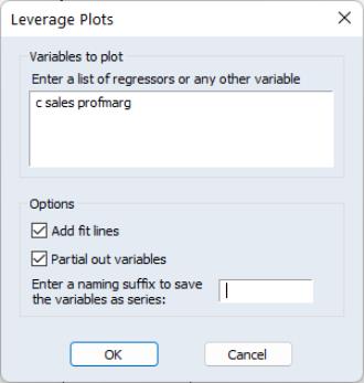
To display leverage plots in EViews select . EViews will then display a dialog which lets you choose some simple options for the leverage plots.
The box lets you enter which variables, or coefficients in a non-linear equation, you wish to plot. By default this box will be filled in with the original regressors from your equation. Note that EViews will let you enter variables that were not in the original equation, in which case the plot will simply show the original equation residuals plotted against the residuals from a regression of the new variable against the original regressors.
To add a regression line to each scatter plot, select the checkbox. If you do not wish to create plots of the partialed variables, but would rather plot the original regression residuals against the raw regressors, unselect the checkbox.
Finally, if you wish to save the partial residuals for each variable into a series in the workfile, you may enter a naming suffix in the box. EViews will then append the name of each variable to the suffix you entered as the name of the created series.
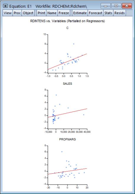
We illustrate using an example taken from Wooldridge (2000, Example 9.8) for the regression of R&D expenditures (RDINTENS) on sales (SALES), profits (PROFITMARG), and a constant (using the workfile “Rdchem.WF1”). The leverage plots for equation E1 are displayed here:
Influence Statistics
Influence statistics are a method of discovering influential observations, or outliers. They are a measure of the difference that a single observation makes to the regression results, or how different an observation is from the other observations in an equation’s sample. EViews provides a selection of six different influence statistics: RStudent, DRResid, DFFITS, CovRatio, HatMatrix and DFBETAS.
• RStudent is the studentized residual; the residual of the equation at that observation divided by an estimate of its standard deviation:
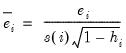 | (26.47) |
where

is the original residual for that observation,

is the variance of the residuals that would have resulted had observation

not been included in the estimation, and

is the
i-th diagonal element of the Hat Matrix,
i.e. 
. The RStudent is also numerically identical to the
t-statistic that would result from putting a dummy variable in the original equation which is equal to 1 on that particular observation and zero elsewhere. Thus it can be interpreted as a test for the significance of that observation.
• DFFITS is the scaled difference in fitted values for that observation between the original equation and an equation estimated without that observation, where the scaling is done by dividing the difference by an estimate of the standard deviation of the fit:
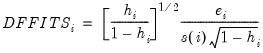 | (26.48) |
• DRResid is the dropped residual, an estimate of the residual for that observation had the equation been run without that observation’s data.
• COVRATIO is the ratio of the determinant of the covariance matrix of the coefficients from the original equation to the determinant of the covariance matrix from an equation without that observation.
• HatMatrix reports the
i-th diagonal element of the Hat Matrix:

.
• DFBETAS are the scaled difference in the estimated betas between the original equation and an equation estimated without that observation:
 | (26.49) |
where

is the original equation’s coefficient estimate, and

is the coefficient estimate from an equation without observation

.
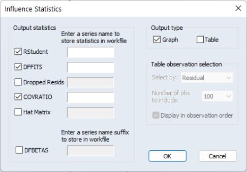
To display influence statistics in EViews select . EViews will bring up a dialog where you can choose how you wish to display the statistics. The box lets you choose which statistics you would like to calculate, and whether to store them as a series in your workfile. Simply check the check box next to the statistics you would like to calculate, and, optionally, enter the name of the series you would like to be created. Note that for the DFBETAS statistics you should enter a naming suffix, rather than the name of the series. EViews will then create the series with the name of the coefficient followed by the naming suffix you provide.
The box lets you select whether to display the statistics in graph form, or in table form, or both. If both boxes are checked, EViews will create a spool object containing both tables and graphs.
If you select to display the statistics in tabular form, then a new set of options will be enabled, governing how the table is formed. By default, EViews will only display 100 rows of the statistics in the table (although note that if your equation has less than 100 observations, all of the statistics will be displayed). You can change this number by changing the dropdown menu. EViews will display the statistics sorted from highest to lowest, where the Residuals are used for the sort order. You can change which statistic is used to sort by using the dropdown menu. Finally, you can change the sort order to be by observation order rather than by one of the statistics by using the check box.
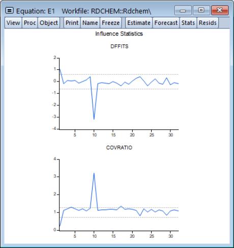
We illustrate using the equation E1 from the “Rdchem.WF1” workfile. A plot of the DFFITS and COVRATIOs clearly shows that observation 10 is an outlier.