Background
A common occurrence in time series regression is the presence of correlation between residuals and their lagged values. This serial correlation violates the standard assumption of regression theory which requires uncorrelated regression disturbances. Among the problems associated with unaccounted for serial correlation in a regression framework are:
• OLS is no longer efficient among linear estimators. Intuitively, since prior residuals help to predict current residuals, we can take advantage of this information to form a better prediction of the dependent variable.
• Standard errors computed using the textbook OLS formula are not correct, and are generally understated.
• If there are lagged dependent variables on the right-hand side of the equation specification, OLS estimates are biased and inconsistent.
A popular framework for modeling serial dependence is the Autoregressive-Moving Average (ARMA) and Autoregressive-Integrated-Moving Average (ARIMA) models popularized by Box and Jenkins (1976) and generalized to Autoregressive-Fractionally Integrated-Moving Average (ARFIMA) specifications.
(Note that ARMA and ARIMA models which allow for explanatory variables in the mean are sometimes termed ARIMAX and ARIMAX. We will generally use ARMA to refer to models both with and without explanatory variables unless there is a specific reason to distinguish between the two types.)
Autoregressive (AR) Models
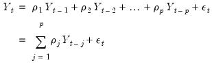
An autoregressive model of order

, denoted AR(

) has the form
 | (24.1) |
where

are the independent and identically distributed innovations for the process and the autoregressive parameters

characterize the na ture of the dependence. Note that the autocorrelations of a stationary AR(

) are infinite, but decline geometrically so they die off quickly, and the partial autocorrelations for lags greater than

are zero.
It will be convenient for the discussion to follow to define a lag operator

such that:
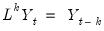 | (24.2) |
and to rewrite the AR(

) as
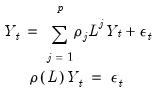 | (24.3) |
where
 | (24.4) |
is a lag polynomial that characterizes the AR process.If we add a mean to the model, we obtain:
 | (24.5) |
The AR(1) Model
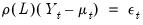
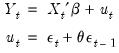
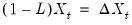
The simplest and most widely used regression model with serial correlation is the first-order autoregressive, or AR(1), model. If the mean

is a linear combination of regressors

and parameters

, the AR(1) model may be written as:
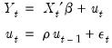 | (24.6) |
The parameter

is the first-order serial correlation coefficient.
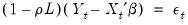
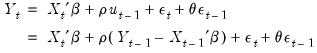
Substituting the second equation into the first, we obtain the regression form
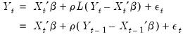 | (24.7) |
In the representation it is easy to see that the AR(1) model incorporates the residual from the previous observation into the regression model for the current observation.
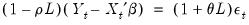
Rearranging terms and using the lag operator, we have the polynomial form
 | (24.8) |
Higher-Order AR Models
A regression model with an autoregressive process of order

, AR(

), is given by:
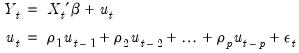 | (24.9) |
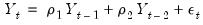
Substituting and rearranging terms, we get the regression
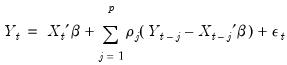 | (24.10) |
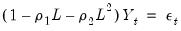
and the polynomial form
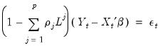 | (24.11) |
Moving Average (MA) Models
A moving average model of order

, denoted MA(

) has the form
 | (24.12) |
where

are the innovations, and
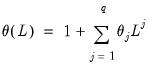 | (24.13) |
is the moving average polynomial with parameters

that characterize the MA process. Note that the autocorrelations of an MA model are zero for lags greater than

.
You should pay particular attention to the definition of the lag polynomial when comparing results across different papers, books, or software, as the opposite sign convention is sometimes employed for the

coefficients.
Adding a mean to the model, we get the mean adjusted form:
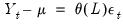 | (24.14) |
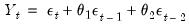
The MA(1) Model
The MA(1) model assumes that the current disturbance term

is a weighted sum of the current and lagged innovations

and

:
 | (24.15) |
The parameter

is the first-order moving average coefficient. Substituting, the MA(1) may be written as
 | (24.16) |
and
 | (24.17) |
Autoregressive Moving Average (ARMA) Models
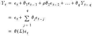
We may combine the AR and the MA specifications to define an autoregressive model moving average (ARMA) model:
 | (24.18) |
We term this model an ARMA(

) to indicate that there are

lags in the AR and

terms in the MA.
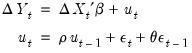
The ARMA(1, 1) Model
The simplest ARMA model is first-order autoregressive with a first-order moving average error:
 | (24.19) |
The parameter

is the first-order serial correlation coefficient, and the

is the moving average coefficient. Substituting, the ARMA(1, 1) may be written as
 | (24.20) |
or equivalently,
 | (24.21) |
Seasonal ARMA Terms
Box and Jenkins (1976) recommend the use of seasonal autoregressive (SAR) and seasonal moving average (SMA) terms for monthly or quarterly data with systematic seasonal movements. Processes with SAR and SMA terms are ARMA models constructed using products of lag polynomials. These products produce higher order ARMA models with nonlinear restrictions on the coefficients.
Seasonal AR Terms
A SAR(

) term is a seasonal autoregressive term with lag

. A SAR adds to an existing AR specification a polynomial with a lag of

:
 | (24.22) |
The SAR is not intended to be used alone. The SAR allows you to form the product of lag polynomials, with the resulting lag structure defined by the product of the AR and SAR lag polynomials.
For example, a second-order AR process without seasonality is given by,
 | (24.23) |
which can be represented using the lag operator

as:
 | (24.24) |
For quarterly data, we might wish to add a SAR(4) term because we believe that there is correlation between a quarter and the quarter the year previous. Then the resulting process would be:
 | (24.25) |
Expanded terms, we see that the process is equivalent to:
 | (24.26) |
The parameter

is associated with the seasonal part of the process. Note that this is an AR(6) process with nonlinear restrictions on the coefficients.
Seasonal MA Terms
Similarly, SMA(

) can be included in your specification to specify a seasonal moving average term with lag

. The resulting the MA lag structure is obtained from the product of the lag polynomial specified by the MA terms and the one specified by any SMA terms.
For example, second-order MA process without seasonality may be written as
 | (24.27) |
or using lag operators:
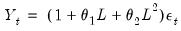 | (24.28) |
To take account of seasonality in a quarterly workfile you may wish to add an SMA(4). Then the resulting process is:
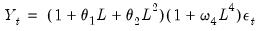 | (24.29) |
The process is equivalent to:
 | (24.30) |
The parameter

is associated with the seasonal part of an MA(6) process which has nonlinear restrictions on the coefficients.
Integrated Models
A time series

is said to be integrated of order 0 or

, if it may be written as a MA process

, with coefficients such that
 | (24.31) |
Roughly speaking, an

process is a moving average with autocovariances that die off sufficiently quickly, a condition which is necessary for stationarity (Hamilton, 2004).

is said to be integrated of order

or

, if its

-th integer difference,

is

, and the

difference is not.
Typically, one assumes that

is an integer and that

or

so that first or second differencing the original series yields a stationary series. We will consider both integer and non-integer integration in turn.
ARIMA Model
An ARIMA(

) model is defined as an

process whose

-th integer difference follows a stationary ARMA(

) process. In polynomial form we have:
 | (24.32) |
Example
The ARIMA(1,1,1) Model
An ARIMA(1,1,1) model for

assumes that the first difference of

is an ARMA(1,1).
 | (24.33) |
Rearranging, and noting that
and
we may write this specification as
 | (24.34) |
or
 | (24.35) |
ARFIMA Model
Stationary processes are said to have long memory when autocorrelations are persistent, decaying more slowly than the rate associated with ARMA models. Modeling long term dependence is difficult for standard ARMA specifications as it requires non-parsimonious, large-order ARMA representations that are generally accompanied by undesirable short-run dynamics (Sowell, 1992).
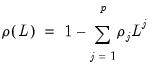
One popular approach to modeling long memory processes is to employ the notion of
fractional integration (Granger and Joyeux, 1980; Hosking, 1981). A fractionally integrated series is one with long-memory that is not

.
Following Granger and Joyeux (1981) and Hosking (1981), we may define a discrete time fractional difference operator which depends on the parameter

:
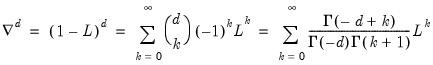 | (24.36) |
for

and

the gamma function.
If the fractional

-difference operator applied to a process produces a random walk we say that the process is an ARFIMA(0,

, 0). Hosking notes that for an ARFIMA(0,

, 0):
• when

, the process is non-stationary but invertible
• when

, the process has long memory but is stationary and invertible
• when

, the process has short memory, with all negative auto-correlations and partial auto correlations, and is invertible
• when

, the process is white noise
More generally, if

-th order fractional differencing results in an ARMA(

), the process is said to be ARFIMA(

). In polynomial form we have:
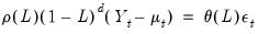 | (24.37) |
Notice that the ARFIMA specification is identical to the standard Box-Jenkins ARIMA formulation in
Equation (24.32), but allowing for non-integer

. Note also that the range restriction on

is non-binding as we may apply integer differencing or summing until

is in the desired range.
By combining fractional differencing with a traditional ARMA specification, the ARFIMA model allows for flexible dynamic patterns. Crucially, when
, the autocorrelations and partial autocorrelations of the ARFIMA process decay more slowly (hyperbolically) than the rates associated with ARMA specifications. Thus, the ARFIMA model allows you to model slowing decaying long-run dependence using the

parameter and more rapidly decaying short-run dynamics using a parsimonious ARMA(

).
The Box-Jenkins (1976) Approach to ARIMA Modeling
In Box-Jenkins ARIMA modeling and forecasting, you assemble a complete forecasting model by using combinations of the three ARIMA building blocks described above. The first step in forming an ARIMA model for a series of residuals is to look at its autocorrelation properties. You can use the correlogram view of a series for this purpose, as outlined in
“Correlogram” .
This phase of the ARIMA modeling procedure is called identification (not to be confused with the same term used in the simultaneous equations literature). The nature of the correlation between current values of residuals and their past values provides guidance in selecting an ARIMA specification.
The autocorrelations are easy to interpret—each one is the correlation coefficient of the current value of the series with the series lagged a certain number of periods. The partial autocorrelations are a bit more complicated; they measure the correlation of the current and lagged series after taking into account the predictive power of all the values of the series with smaller lags. The partial autocorrelation for lag 6, for example, measures the added predictive power of

when

are already in the prediction model. In fact, the partial autocorrelation is precisely the regression coefficient of

in a regression where the earlier lags are also used as predictors of

.
If you suspect that there is a distributed lag relationship between your dependent (left-hand) variable and some other predictor, you may want to look at their cross correlations before carrying out estimation.
The next step is to decide what kind of ARIMA model to use. If the autocorrelation function dies off smoothly at a geometric rate, and the partial autocorrelations were zero after one lag, then a first-order autoregressive model is appropriate. Alternatively, if the autocorrelations were zero after one lag and the partial autocorrelations declined geometrically, a first-order moving average process would seem appropriate. If the autocorrelations appear to have a seasonal pattern, this would suggest the presence of a seasonal ARMA structure. Along these lines, Box and Jenkins (1976) recommend the use of seasonal autoregressive (SAR) and seasonal moving average (SMA) terms for monthly or quarterly data with systematic seasonal movements.
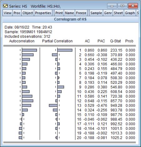
For example, we can examine the correlogram of the DRI Basics housing series in the “Hs.WF1” workfile by setting the sample to “1959m01 1984m12” then selecting from the HS series toolbar. Click on to accept the default settings and display the result.
The “wavy” cyclical correlogram with a seasonal frequency suggests fitting a seasonal ARMA model to HS.
The goal of ARIMA analysis is a parsimonious representation of the process governing the residual. You should use only enough AR and MA terms to fit the properties of the residuals. The Akaike information criterion and Schwarz criterion provided with each set of estimates may also be used as a guide for the appropriate lag order selection.
After fitting a candidate ARIMA specification, you should verify that there are no remaining autocorrelations that your model has not accounted for. Examine the autocorrelations and the partial autocorrelations of the innovations (the residuals from the ARIMA model) to see if any important forecasting power has been overlooked. EViews provides several views for diagnostic checks after estimation.