Estimation Method Details
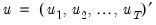
In
“ARMA Method” we described how EViews lets you choose between maximum likelihood (ML), generalized least squares (GLS), and conditional least squares (CLS) estimation for ARIMA and ARFIMA estimation.
Recall that for the general ARIMA(

) model we have
 | (24.52) |
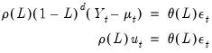
for the unconditional residuals
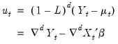 | (24.53) |
and innovations
 | (24.54) |
We will use the expressions for the unconditional residuals and innovations to describe three objective functions that may be used to estimate the ARIMA model.
(For simplicity of notation our discussion abstracts from SAR and SMA terms and coefficients. It is straightforward to allow for the inclusion of these seasonal terms).
Maximum Likelihood (ML)
Estimation of ARIMA and ARFIMA models is often performed by exact maximize likelihood assuming Gaussian innovations.
The exact Gaussian likelihood function for an ARIMA or ARFIMA model is given by
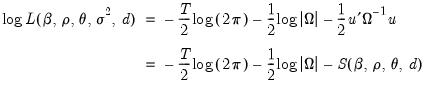 | (24.55) |
where
and
, where

is the symmetric Toeplitz covariance matrix for the

draws from the ARMA/ARFIMA process for the unconditional residuals (Doornik and Ooms 2003). Note that direct evaluation of this function requires the inversion of a large

matrix

which is impractical for large

for both storage and computational reasons.
The ARIMA model restricts

to be a known integer. The ARFIMA model treats

as an estimable parameter.
ARIMA ML
It is well-known that for ARIMA models where

is a known integer, we may employ the Kalman filter to efficiently evaluate the likelihood. The Kalman filter works with the state space prediction error decomposition form of the likelihood, which eliminates the need to invert the large matrix

.
See Hamilton (2004, Chapter 13, p. 372) or Box, Jenkins, and Reinsel (2008, 7.4, p. 275) for extensive discussion.
ARFIMA ML
Sowell (1992) and Doornik and Ooms (2003) offer detailed descriptions of the evaluation of the likelihood for ARFIMA models. In particular, practical evaluation of
Equation (24.55) requires that we address several computational issues.
First, we must compute the autocovariances of the ARFIMA process that appear in the

which an involve an infinite order MA representation. Fortunately, Hosking (1981) and Sowell (1992) describe closed-form alternatives and Sowell (1992) derives efficient recursive algorithms using hypergeometric functions.
Second, we must compute the determinant of the variance matrix and generalized (inverse variance weighted) residuals in a manner that is computationally and storage efficient. Doornik and Ooms (2003) describe a Levinson-Durbin algorithm for efficiently performing this operation with minimal operation count while eliminating the need to store the full

matrix

.
Third, where possible we follow Doornik and Ooms (2003) in concentrate the likelihood with respect to the regression coefficients

and the scale parameter

.
Generalized Least Squares (GLS)
Since the exact likelihood function in
Equation (24.55) depends on the data, and the mean and ARMA parameters only through the last term in the expression, we may ignore the inessential constants and the log determinant term to define a generalized least squares objective function
 | (24.56) |
and the ARFIMA estimates may be obtained by minimizing

.
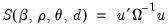
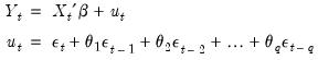
Conditional Least Squares (CLS)
Box and Jenkins (1976) and Box, Jenkins, and Reinsel (2008, Section 7.1.2 p 232.) point out that conditional on pre-sample values for the AR and MA errors, the normal conditional likelihood function may be maximized by minimizing the sum of squares of the innovations.
The recursive innovation equation in
Equation (24.54) is easy to evaluate given parameter values, lagged values of the differenced

,

, and estimates of the lagged innovations. Note, however that neither the

nor the can be substituted in the first period as they are not available until we start up the difference equation.
We discuss below methods for starting up the recursion by specifying presample values of

and

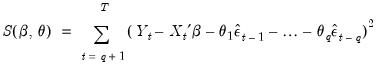
. Given these presample values, the conditional likelihood function for normally distributed innovations is given by
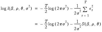 | (24.57) |
Notice that the conditional likelihood function depends on the data and the mean and ARMA parameters only through the conditional least squares function

, so that the conditional likelihood may be maximized by minimizing

.
Coefficient standard errors for the CLS estimation are the same as those for any other nonlinear least squares routine: ordinary inverse of the estimate of the information matrix, or a White robust or Newey-West HAC sandwich covariance estimator. In all three cases, one can use either the Gauss-Newton outer-product of the Jacobians, or the Newton-Raphson negative of the Hessian to estimate the information matrix.
In the remainder of this section we discuss the initialization of the recursion. EViews initializes the AR errors using lagged data (adjusting the estimation sample if necessary), and initializes the MA innovations using backcasting or the unconditional (zero) expectation.
Initializing the AR Errors
Consider an AR(

) regression model of the form:
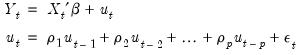 | (24.58) |
for
. Estimation of this model using conditional least squares requires computation of the innovations

for each period in the estimation sample.
We can rewrite out model as
 | (24.59) |
so we can see that we require

pre-sample values to evaluate the AR process at

Typically conditional least squares employs lagged values of the variables in the model to initialize the process. For example, to estimate an AR(1) model, one may transforms the linear model,
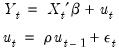 | (24.60) |
into a nonlinear model by substituting the second equation into the first, writing

in terms of observables and rearranging terms:
 | (24.61) |
so that the innovation recursion written in terms of observables is given by
 | (24.62) |
Notice that we require observation on the

and

in the period before the start of the recursion. If these values are not available, we must adjust the period of interest to begin at

so that the values of the observed data in

may be substituted into the equation to obtain an expression for

.
Higher order AR specifications are handled analogously. For example, a nonlinear AR(3) is estimated using nonlinear least squares on the innovations given by:
 | (24.63) |
It is important to note that textbooks often describe techniques for estimating linear AR models like
Equation (24.58). The most widely discussed approaches, the Cochrane-Orcutt, Prais-Winsten, Hatanaka, and Hildreth-Lu procedures, are multi-step approaches designed so that estimation can be performed using standard linear regression. These approaches proceed by obtaining an initial consistent estimate of the AR coefficients

and then estimating the remaining coefficients via a second-stage linear regression.
All of these approaches suffer from important drawbacks which occur when working with models containing lagged dependent variables as regressors, or models using higher-order AR specifications; see Davidson and MacKinnon (1993, p. 329–341), Greene (2008, p. 648–652).
In contrast, the EViews conditional least squares estimates the coefficients

and

are estimated simultaneously by minimizing the nonlinear sum-of-squares function

(which maximizes the conditional likelihood). The nonlinear least squares approach has the advantage of being easy-to-understand, generally applicable, and easily extended to models that contain endogenous right-hand side variables and to nonlinear mean specifications.
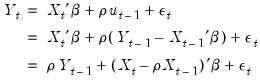
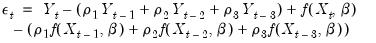
Thus, for a nonlinear mean AR(1) specification, EViews transforms the nonlinear model,
 | (24.64) |
into the alternative nonlinear regression form
 | (24.65) |
yielding the innovation specification:
 | (24.66) |
Similarly, for higher order ARs, we have:
 | (24.67) |
For additional detail, see Fair (1984, p. 210–214), and Davidson and MacKinnon (1993, p. 331–341).
Initializing MA Innovations
Consider an MA(

) regression model of the form:
 | (24.68) |
for

. Estimation of this model using conditional least squares requires computation of the innovations

for each period in the estimation sample.
Computing the innovations is a straightforward process. Suppose we have an initial estimate of the coefficients,

, and estimates of the pre-estimation sample values of

:
 | (24.69) |
Then, after first computing the unconditional residuals
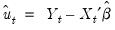
, we may use forward recursion to solve for the remaining values of the innovations:
 | (24.70) |
for

.
All that remains is to specify a method of obtaining estimates of the pre-sample values of

:
 | (24.71) |
One may employ backcasting to obtain the pre-sample innovations (Box and Jenkins, 1976). As the name suggests, backcasting uses a backward recursion method to obtain estimates of

for this period.
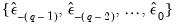
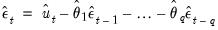
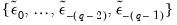
To start the recursion, the

values for the innovations
beyond the estimation sample are set to zero:
 | (24.72) |
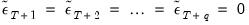
EViews then uses the actual results to perform the backward recursion:
 | (24.73) |
for
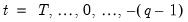
. The final

values,
, which we use as our estimates, may be termed the backcast estimates of the pre-sample innovations. (Note that if your model also includes AR terms, EViews will

-difference the

to eliminate the serial correlation prior to performing the backcast.)
Alternately, one obvious method is to turn backcasting off and to set the pre-sample

to their unconditional expected values of 0:
 | (24.74) |
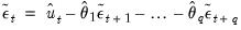
Whichever methods is used to initialize the presample values, the sum-of-squared residuals (SSR) is formed recursively as a function of the

and

, using the fitted values of the lagged innovations:
 | (24.75) |
and the expression is minimized with respect to

and

.
The backcast step, forward recursion, and minimization procedures are repeated until the estimates of

and

converge.