An Illustration
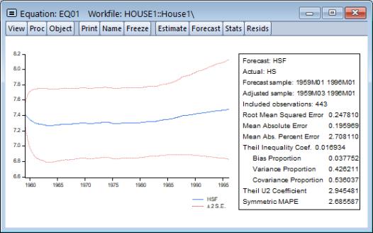
Suppose we produce a dynamic forecast using EQ01 over the sample 1959M01 to 1996M01. The forecast values will be placed in the series HSF, and EViews will display a graph of the forecasts and the plus and minus two standard error bands, as well as a forecast evaluation:
This is a dynamic forecast for the period from 1959M01 through 1996M01. For every period, the previously forecasted values for HS(-1) are used in forming a forecast of the subsequent value of HS. As noted in the output, the forecast values are saved in the series HSF. Since HSF is a standard EViews series, you may examine your forecasts using all of the standard tools for working with series objects.
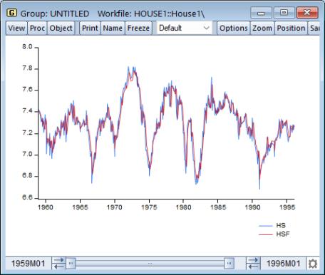
For example, we may examine the actual versus fitted values by creating a group containing HS and HSF, and plotting the two series. Select HS and HSF in the workfile window, then right-mouse click and select . Then select and select Line & Symbolin the page to display a graph of the two series:
Note the considerable difference between this actual and fitted graph and the depicted above.
To perform a series of one-step ahead forecasts, click on on the equation toolbar, and select Static forecast. Make certain that the forecast sample is set to “1959m01 1995m06”. Click on . EViews will display the forecast results:
We may also compare the actual and fitted values from the static forecast by examining a line graph of a group containing HS and the new HSF.
The one-step ahead static forecasts are more accurate than the dynamic forecasts since, for each period, the actual value of HS(‑1) is used in forming the forecast of HS. These one-step ahead static forecasts are the same forecasts used in the displayed above.
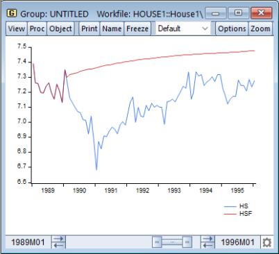
Lastly, we construct a dynamic forecast beginning in 1990M02 (the first period following the estimation sample) and ending in 1996M01. Keep in mind that data are available for SP for this entire period. The plot of the actual and the forecast values for 1989M01 to 1996M01 is given by:
Since we use the default settings for out-of-forecast sample values, EViews backfills the forecast series prior to the forecast sample (up through 1990M01), then dynamically forecasts HS for each subsequent period through 1996M01. This is the forecast that you would have constructed if, in 1990M01, you predicted values of HS from 1990M02 through 1996M01, given knowledge about the entire path of SP over that period.
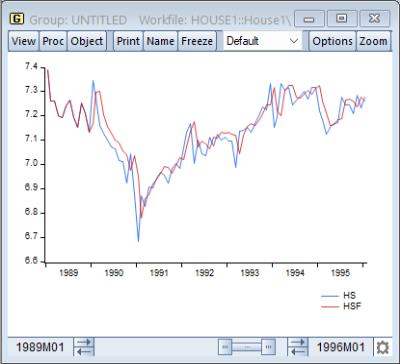
The corresponding static forecast is displayed below:
Again, EViews backfills the values of the forecast series, HSF1, through 1990M01. This forecast is the one you would have constructed if, in 1990M01, you used all available data to estimate a model, and then used this estimated model to perform one-step ahead forecasts every month for the next six years.
The remainder of this chapter focuses on the details associated with the construction of these forecasts, the corresponding forecast evaluations, and forecasting in more complex settings involving equations with expressions or auto-updating series.