Forecasting from an Estimated Equation
We have been working with a subset of our data, so that we may compare forecasts based upon this model with the actual data for the post-estimation sample 1993Q1–1996Q4.
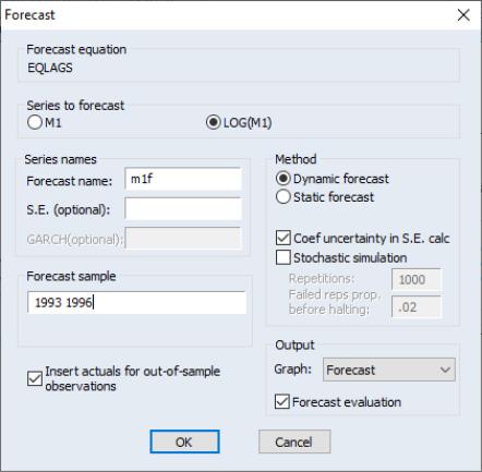
Click on the button in the EQLAGS equation toolbar to open the forecast dialog:
We set the forecast sample to 1993Q1–1996Q4 and provide names for both the forecasts and forecast standard errors so both will be saved as series in the workfile. The forecasted values will be saved in M1_F and the forecast standard errors will be saved in M1_SE.
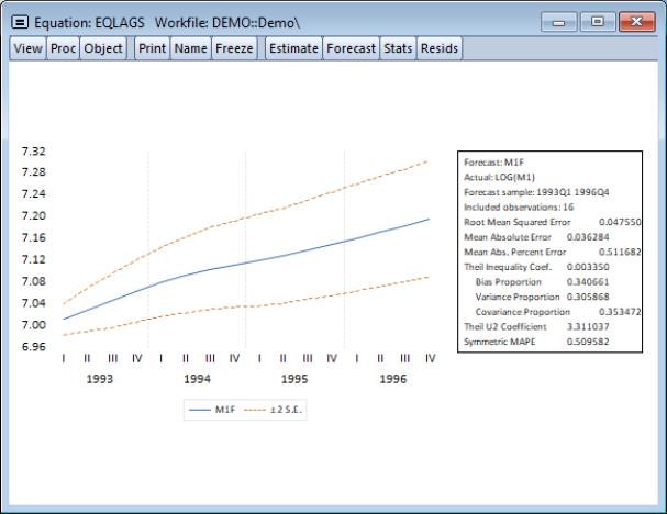
Note also that we have elected to forecast the log of M1, not the level, and that we request both graphical and forecast evaluation output. The option constructs the forecast for the sample period using only information available at the beginning of 1993Q1. When you click , EViews displays both a graph of the forecasts, and statistics evaluating the quality of the fit to the actual data:
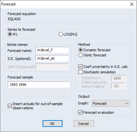
Alternately, we may also choose to examine forecasts of the level of M1. Click on the button in the EQLAGS toolbar to open the forecast dialog, and select under the Series to forecast option. Enter a new name to hold the forecasts and standard errors, say M1LEVEL_F and M1LEVEL_SE, and click .
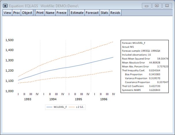
EViews will present a graph of the forecast of the level of M1, along with the asymmetric confidence intervals for this forecast:
The series that the forecast procedure generates are ordinary EViews series that you may work with in the usual ways. For example, we may use the forecasted series for LOG(M1) and the standard errors of the forecast to plot actuals against forecasted values with (approximate) 95% confidence intervals for the forecasts.
We will first create a new group object containing these values. Select from the main menu, and enter the expressions:
m1_f+2*m1_se m1_f-2*m1_se log(m1)
to create a group containing the confidence intervals for the forecast of LOG(M1) and the actual values of LOG(M1):
There are three expressions in the dialog. The first two represent the upper and lower bounds of the (approximate) 95% forecast interval as computed by evaluating the values of the point forecasts plus and minus two times the standard errors. The last expression represents the actual values of the dependent variable.
When you click , EViews opens an untitled group window containing a spreadsheet view of the data. Before plotting the data, we will change the sample of observations so that we only plot data for the forecast sample. Select or click on the button in the group toolbar, and change the sample to include only the forecast period:
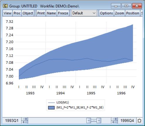
To plot the data for the forecast period, select from the group window and choose Mixed from the list on the left of the Graph Options dialog, then go to the node, set the first two entries to and the last entry to :
The actual values of log(M1) are depicted using the line, and the area band shows the approximate 95% confidence interval.
(Note that the slider bar at the bottom of the graph indicates that we are viewing only a subset of the workfile range).
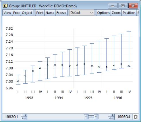
For an alternate view of these data, you can select from the list in the dialog, which displays the graph as follows:
This graph shows clearly that the forecasts of LOG(M1) over-predict the actual values in the last four quarters of the forecast period.