Example
We consider here an example of LSTAR estimation using a multiple equilibrium model of unemployment and data described in Martin, Hurn, and Harris (2013, 19.9.1, p. 744). The model is a simple two-regime error correction model of the change in the unemployment rate

:
 | (36.16) |
where
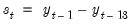
is the lagged annual change in the rate.
The data for unemployment consist of the U.S. Civilian Unemployment Rate (UNRATE) for persons 16 and older from 1948m01 to 2010m03 (2010-10-08 vintage). The “unemp_mhh19.wf1” workfile containing these data obtained from BLS is available in your EViews example data.
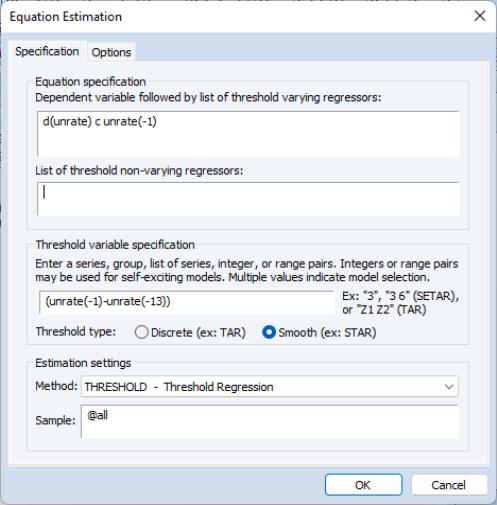
To estimate this model, open the smooth threshold dialog and fill it out as depicted:
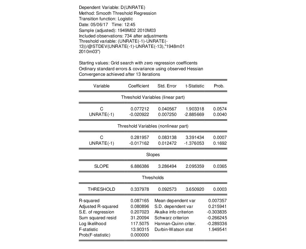
We can leave the options at their default values. Click on to estimate this specification and display the results.
Comparison of these results to those reported in Table 19.6 of Martin, Hurn, and Harris shows that while the estimates of the

and

match, the estimates of the smoothing function slope parameter does not match. This difference stems from the fact that like some authors, Martin, Hurn, and Harris estimate the threshold weighting function employing a scaling factor

equal to the sample standard deviation of the threshold variable. The resulting parameterization is given by
 | (36.17) |
We can obtain the equivalent result by dividing the estimator of

and its corresponding standard error by the standard deviation of the threshold, or we can modify the existing specification to account for the weighting.
We can modify our estimates to match the weighted

results by either by creating a new scaled threshold series, or by directly entering the scaled expression
(unrate(-1)-unrate(-13))/@stdev(unrate(-1)-unrate(-13))
in the dialog and estimating the resulting specification:
The slopes now match, but the new estimates of

do not.We can obtain equivalent results for

by multiplying by the standard error by the standard deviation of the threshold.
It is worth commenting that the reason that some authors perform this scaling is to improve the numeric stability of the estimator procedure. We note that EViews always scales internally, but displays the results in the original metric.
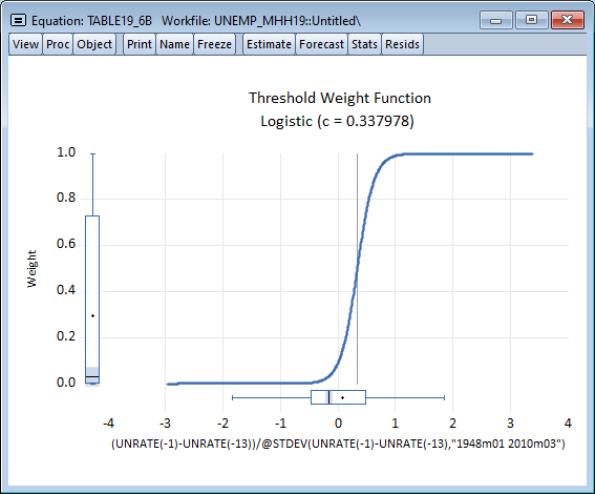
We may display the transition function by clicking on , and clicking on to accept the default settings:
Visually, we see that the median transition weight is near 0.3 and that the upper end of the IQR only extends to around 0.75. Moreover, the weight function is rather steep, with most of the variation occurring well within one standard deviation of the lagged annual change in the rate.
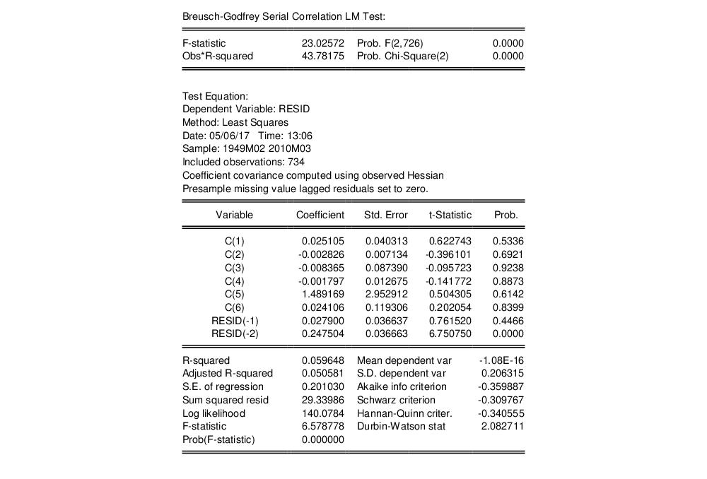
Clicking on and accepting the defaults, computes a Breusch-Godfrey serial correlation LM test using a default lag of 2:
There is strong evidence against the null of no serial correlation, suggesting that the lag structure of the STAR is insufficient to account for autocorrelation.
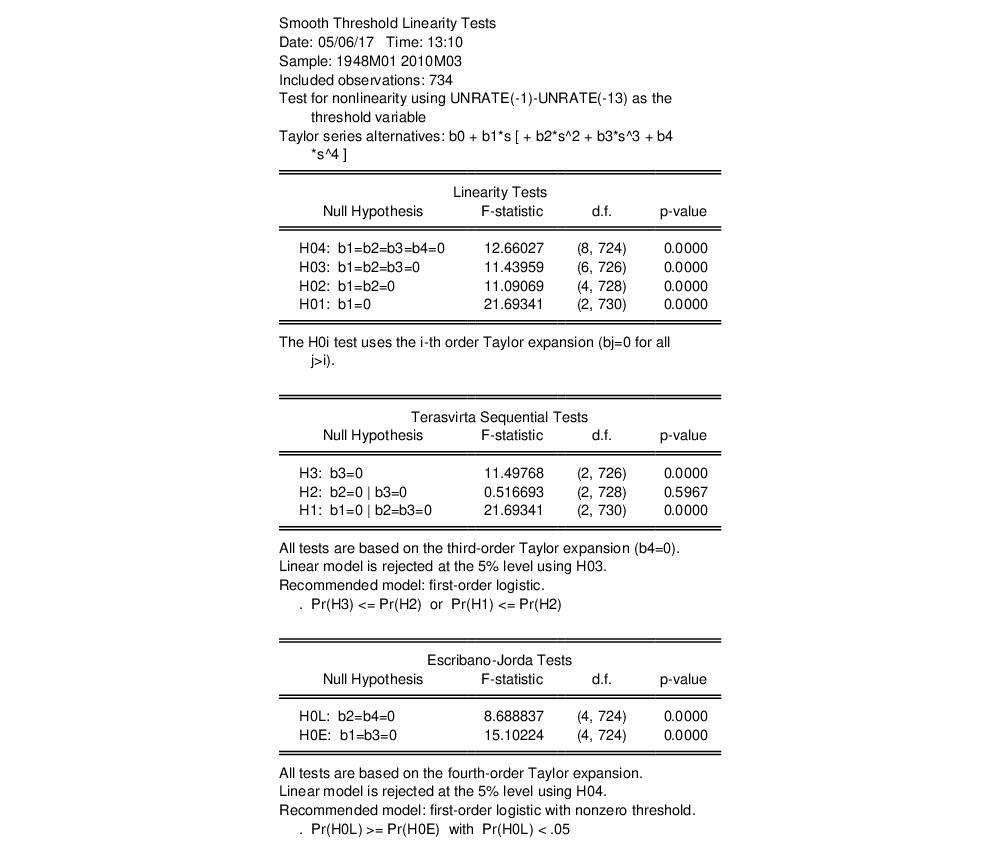
We may perform a linearity test by clicking on :
The tests strongly reject the null of linearity against the smooth transition alternatives. Moreover, both the Terasvirta and the Escribano-Jordan discrimination tests favor the logistic threshold function.
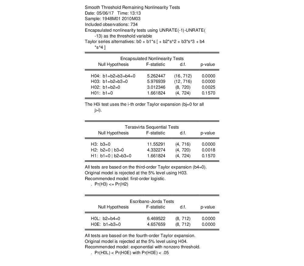
We may test against remaining nonlinearity using either the additive or encapsulated nonlinearity tests. Performing the encapsulated test by selecting yields:
suggesting that the current model is inadequate to capture the nonlinear dynamics.