Estimation Output
EViews displays a variety of results in the output view following estimation.
The top portion of the output displays information about the optimization technique, ARMA estimation method, the coefficient covariance calculation, and if requested, the starting values used to initialize the optimization procedure.
The next section shows the estimated coefficients, coefficient standard errors, and t-statistics. In addition to the estimates of the ARMA coefficients, EViews will display estimates of the fractional integration parameter for ARFIMA models, and the estimate of the error variance if the ARMA estimation method is maximum likelihood, labeled SIGMASQ.
All of these results may be interpreted in the usual manner.
In the section directly below the coefficient estimates are the usual descriptive statistics for the dependent variable, along with a variety of summary and descriptive statistics for the estimated equation.
Note that all of the equation summary results involving residuals differ from those computed in standard OLS settings so that some care should be taken in interpreting results. To understand the issues, keep in mind that there are two different residuals associated with an ARMA model. The first are the estimated unconditional residuals:
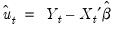 | (24.47) |
which are computed using the original explanatory variables and the estimated coefficients,

. These residuals are the errors that you would obtain if you made a prediction of the value of

using contemporaneous information while ignoring the information contained in the lagged residuals.
Generally, there is little reason to examine the unconditional residuals, and EViews does not automatically compute them following estimation.
The second set of residuals are the estimated
one-period ahead forecast errors,

. As the name suggests, these residuals represent the forecast errors you would make if you computed forecasts using a prediction of the residuals based upon past values of your data, in addition to the contemporaneous information. In essence, you improve upon the unconditional forecasts and residuals by taking advantage of the predictive power of the lagged residuals.
For ARMA models, the computed residuals, and all of the residual-based regression statistics—such as the

, the standard error of regression, and the Durbin-Watson statistic— reported by EViews are based on the estimated one-period ahead forecast errors,

.
Lastly, to aid in the interpretation of the results for ARMA and ARFIMA models, EViews displays a the reciprocal roots of the AR and MA polynomials in the lower block of the results. EViews reports these roots as
Inverted AR Roots and at the bottom of the regression output. For our general ARMA model with the lag polynomials

and

, the reported roots are the roots of the polynomials:
 | (24.48) |
The roots, which may be imaginary, should have modulus no greater than one. The output will display a warning message if any of the roots violate this condition.
If

has a real root whose absolute value exceeds one or a pair of complex reciprocal roots outside the unit circle (that is, with modulus greater than one), it means that the autoregressive process is explosive.
For example, in the simple AR(1) model, the estimated parameter

is the serial correlation coefficient of the unconditional residuals. For a stationary AR(1) model, the true

lies between –1 (extreme negative serial correlation) and +1 (extreme positive serial correlation).
If

has reciprocal roots outside the unit circle, we say that the MA process is
noninvertible, which makes interpreting and using the MA results difficult. However, noninvertibility poses no substantive problem, since as Hamilton (1994a, p. 65) notes, there is always an equivalent representation for the MA model where the reciprocal roots lie inside the unit circle. Accordingly, you should try to re-estimate your model with different starting values until you get a moving average process that satisfies invertibility. Alternatively, you may wish to turn off MA backcasting (see
“Initializing MA Innovations”).
If the estimated MA process has roots with modulus close to one, it is a sign that you may have over-differenced the data, which introduced an MA unit root. The process will be difficult to estimate and even more difficult to forecast. If possible, you should re-estimate with one less round of differencing, perhaps using ARFIMA to account for long-run dependence.
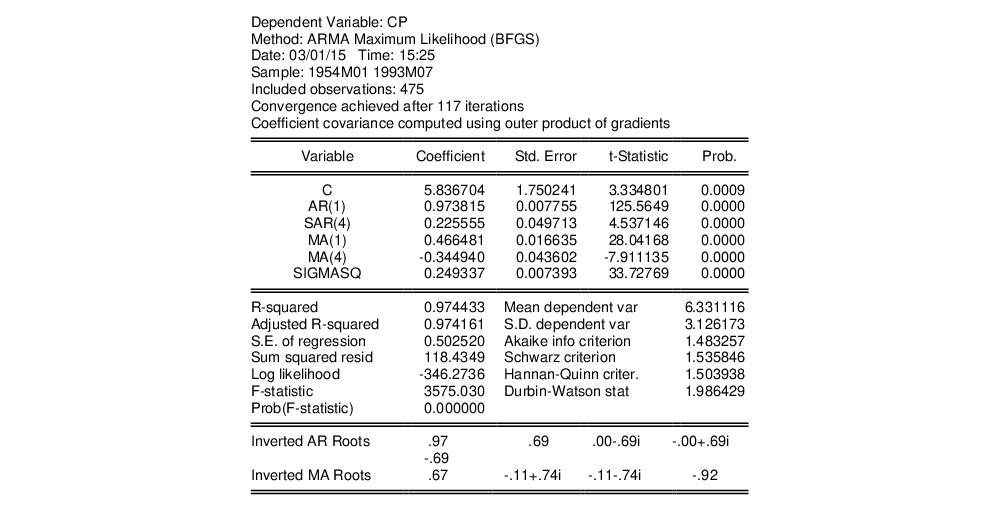
Consider the following example output from ARMA estimation:
This estimation result corresponds to the following specification,
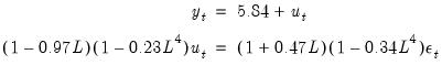 | (24.49) |
or equivalently, to:
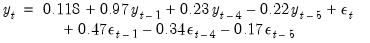 | (24.50) |
Note the signs of the MA terms, which may be reversed from those in some textbooks. Note also that the inverted AR roots have moduli very close to one, which is typical for many macro time series models.