Examples
To illustrate the estimation of ARIMA and ARFIMA specifications in EViews we consider examples from Sowell (1992a) which model the natural logarithm of postwar quarterly U.S. real GDP from 1947q1 to 1989q4. Sowell estimates a number of models which are compared using AIC and SIC. We will focus on the ARMA(3, 2) and ARFIMA(3,

, 2) specifications (Table 2, p. 288 and Table 3, p. 289).
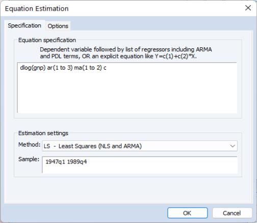
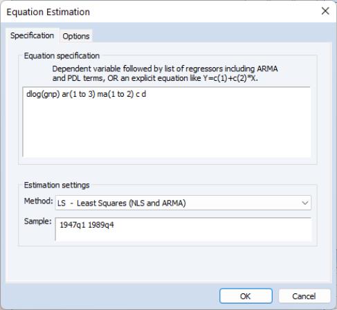
To estimate the ARMA(3, 2) we open an equation dialog by selecting , by selecting , or by typing the command keyword equation in the command line. EViews will display the least squares dialog:
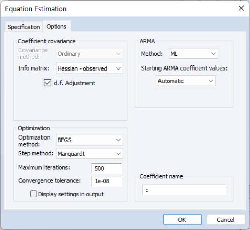
We enter the expression for the dependent variable, followed by the AR and MA terms using ranges that include all of the desired terms, and C to indicate that we wish to include an intercept. Next, we click on the tab to display the estimation settings.
First, we instruct EViews to compute coefficient standard errors using the observed Hessian by setting the Information matrix dropdown to . In addition, we set the to , the to “1e-8”, and the to . Click on to estimate the model.
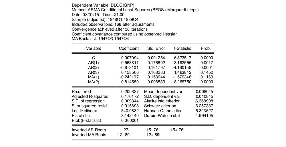
EViews will perform the iterative maximum likelihood estimation using BFGS and will display the estimation results:
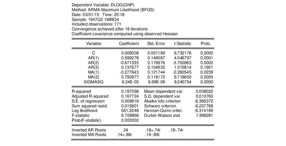
The top portion of the output displays information about the estimation method, optimization, and covariance calculation.
The next section contains the coefficient estimates, standard errors, t-statistics and corresponding p-value. (It is worth pointing out that the reported ARMA coefficients use a different sign convention than those in Sowell so that the ARMA coefficients all have the opposite sign).
Notice that since we estimated the model using ML, EViews displays the estimate of the error variance as one of the estimated coefficients. You should be aware that the EViews reported p-value for SIGMASQ is for the two-sided test, despite the fact that SIGMASQ must be non-negative. (If desired, you may use the reported coefficient, standard error, and the @CTDIST function to compute the appropriate one-sided p-value.)
The final section shows the inverted AR and MA roots.
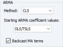
It may be instructive to compare these results to those obtained from an alternative conditional least squares approach to estimating the specification. To reestimate your equation using CLS, click on the button to bring up the dialog, then on the tab to show the estimation options. In the section of the page, we have:
Select in the dropdown, and click on to estimate the new specification.
Click on to accept the changes and re-estimate the model.
The top of the new equation output now reports that estimation was performed using CLS and that the MA errors were initialized using backcasting. Despite the different objectives, we see that the CLS ARMA coefficient estimates are generally quite similar to those obtained from exact ML estimation. Lastly, we note that the estimate of the variance is not reported as part of the coefficient output for CLS estimation.
Next, following Sowell, we estimate an ARFIMA(3,

, 2). Once again, click on the button to bring up the dialog:
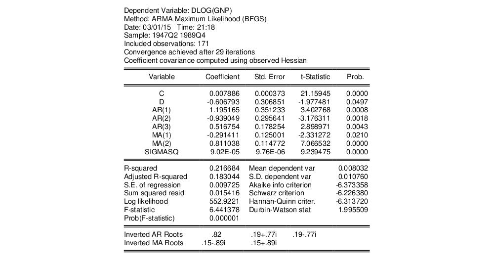
and add the special d keyword to the list of regressors to tell EViews that you wish to estimate the fractional integration parameter. Click on to estimate the updated equation.
Notice first that EViews has switched from CLS estimation to ML since ARFIMA models may only be estimated using ML or GLS.
Turning to the estimate of the fractional differencing parameter, we see that it is negative and statistically significantly different from zero at the 5% level. Thus, we can reject the unit root hypothesis under this specification. Alternately, we cannot reject the time trend null hypothesis that

.
(Note: the results reported in Sowell differ slightly, presumably due to differences in the nonlinear optimization procedure in general, and the estimate of the observed Hessian in particular—for what it is worth, the EViews likelihood is slightly higher than the likelihood reported by Sowell. Notably, Sowell’s conclusions differ slightly from than those outlined here, as he finds that the unit root and trend hypotheses are both consistent with the ARFIMA estimates. Sowell does not reject the zero null at the 5% level, but does reject at the 10% level. See Sowell for detailed interpretation of results.)