EViews 9.5 MIDAS Forecasting Demonstration

Traditional approaches to time-series estimation and forecasting in economics require that the variables be of the same frequency. This often causes a problem since most macroeconomic data is reported at different intervals and frequencies. For example in many countries GDP is reported on a quarterly basis, whereas unemployment figures are reported monthly, and interest rates or stock market prices are reported daily. A frequently used solution to this issue has been to aggregate the higher frequency data into values in the lower frequency. For example, the 3 months of unemployment data in each quarter are averaged to give a single quarterly value. A significant disadvantage to this approach is that through the aggregation you discard data which can lead to less accurate estimation.

Mixed-Data Sampling (MIDAS) is a method of estimating and forecasting from models where the dependent variable is recorded at a lower frequency than one or more of the independent variables. Unlike the traditional aggregation approach, MIDAS uses information from every observation in the higher frequency space.

As an example of using MIDAS in EViews, we will follow the Federal Reserve Bank of St Louis paper "Forecasting with Mixed Frequencies" from November 2010. In one of the applications in this paper, the authors forecast quarterly GDP rates using monthly employment growth data. We will perform a similar study using more recent data.

First we need to obtain the data in an EViews workfile. We will create a workfile with a quarterly page and a monthly page. For our study we will be using data from 1985 onwards. We click on File–>New–>Workfile, and then change the Frequency to Quarterly and enter the required dates. We will give the page the name GDPQuart:

Clicking OK will create the specified workfile.

To create the monthly page we click on the New Page tab at the bottom of our workfile and select Specify by Frequency/Range … This will bring up the same dialog as we just used, but this time we will select Monthly as the Frequency, and name the page EMPMonth. Clicking OK gives us a two page workfile:

Next we use the convenient FRED interface to search for and fetch the GDP and employment data. We click on File–>Open–>Database, and then select FRED Database as the Database Type and then click OK. This opens a connection to the FRED database. To browse through the available data, we click the Browse button. To search for GDP we select All Series Search, then enter GDP in the search box:

Since we are interested in nominal GDP, we’ll use the second result. To import the data into our workfile we can simply drag the icon onto our quarterly page.

Double clicking the gdp icon lets us view the data. We see that we have data for GDP from 1985 until 2015Q3:

To search for an employment series we will type employment in the FRED search box:

The third result, Total Nonfarm Payrolls is the result we require. We will drag its icon onto our monthly workfile page. If we open up the series, we can see we have data until 2015M12.

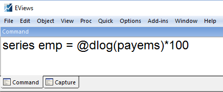
Following the original Federal Reserve paper, we will create transformations of the GDP and employment data to produce growth rates. Using the EViews command line, we first (ensuring that we currently have the monthly page open) enter a command to calculate the log-difference of payrolls, multiplied by one hundred:

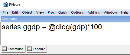
Switching to the Quarterly page, we calculate a growth rate for GDP:

Now we have our data we can estimate our first equation. To begin we will estimate a model using the traditional aggregation technique for dealing with different frequency regressors; a simple equation regressing GDP Growth against a constant, a single lag of GDP Growth and the aggregation of monthly employment growth, lagged 1 quarter. We switch to our quarterly page and click on Quick–>Estimate Equation and enter our equation specification.

Note that EViews allows you to directly specify variables from other pages inside the equation specification using the pagename\seriesname syntax. EViews will aggregate the monthly values of employment automatically for us. Clicking OK produces the estimation results:

Since we only have data for employment through 2015M12 (i.e. Q4), we can only estimate this equation using data through 2015Q3. We can see that the estimate of the constant is around 0.8, and the lag of GDP growth is around 0.16, although slightly insignificant at a 10% level.

Clicking on the Name button allows us to name our equation EQ01.

Our second equation will use an Almon/PDL lag weighted MIDAS regression. We again click on Quick–>Estimate Equation to bring up the estimation dialog. We change the Method: dropdown to select MIDAS. We enter our dependent variable, GDP growth along with a constant and a lag of GDP growth in the first specification box. The second box allows us to enter our monthly regressor, again using the syntax pagename\seriesname. We enter monemp\emp(-5). The -5 signifies that we want the employment values lagged by 5 months. EViews calculates the lags starting from the last month of the quarter. The Federal Reserve paper uses data from the first month of the previous quarter, so to match up we need to take a 5 month lag.

The Almon MIDAS method takes a number of periods of the higher frequency variable and fits them to a lower-order polynomial. We simply need to specify how many periods of monthly employment will be used in the polynomial. EViews allows you to set a fixed number of periods (lags), or choose automatically. To match the Federal Reserve paper, we will fix it at 9:

Clicking OK produces the results:

The results are split into three sections – we have:

• the quarterly coefficients at the top.

• the polynomial coefficients in the middle.

• the individual lag coefficients at the bottom.

We can see that the coefficient on the constant term is similar to our previous estimation, and the coefficient on the lag of GDP growth is slightly higher, and more significant.

We again click the Name button to give our equation a name, EQ02.

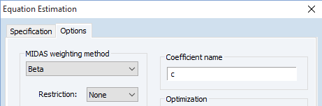
Our third equation will use a Step weighted MIDAS regression. We follow the same steps as the previous equation, but use the Options tab of the estimation dialog to change the MIDAS weight method:

The results from this estimation are similar to the previous:

The coefficients on the constant and the lag of GDP growth are very similar to our previous estimation. We name this estimation EQ03.

Our final estimation will use a Beta weighted MIDAS regression with no restrictions. This is estimated in the same way as the previous two regressions, but we change the MIDAS weight to Beta:

Having estimated our 4 equations for GDP growth, we’ll use EViews’ forecast averaging tool to create a combination of forecasts of GDP growth through 2016Q1 – i.e. a forecast of two quarters. To do this we open up the GDPG series and click on Proc–>Forecast Averaging ... EViews allows us to use the existing equation objects to perform the forecasts to be combined. We simply need to enter the name of the equation objects in the Forecast data objects box, then specify the sample we wish to forecast over and the type of averaging method we want to use (we will stick with a simple mean calculation):

Clicking OK produces the averaging output:

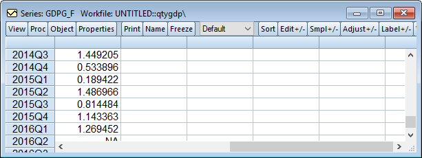
The multiple lines during the forecast period represent each of the individual forecasts and their average. The red line is the non-MIDAS aggregation approach, and it clearly produces a forecast much higher than the MIDAS estimations. Opening the generated series GDPG_F, we can view the actual data of the forecast (note that the values prior to 2015Q4 are the actual data values):