Forecasting from Equations with Expressions
One of the most useful EViews innovations is the ability to estimate and forecast from equations that are specified using expressions or auto-updating series. You may, for example, specify your dependent variable as LOG(X), or use an auto-updating regressor series EXPZ that is defined using the expression EXP(Z). Using expressions or auto-updating series in equations creates no added complexity for estimation since EViews simply evaluates the implicit series prior to computing the equation estimator.
The use of expressions in equations does raise issues when computing forecasts from equations. While not particularly complex or difficult to address, the situation does require a basic understanding of the issues involved, and some care must be taken when specifying your forecast.
In discussing the relevant issues, we distinguish between specifications that contain only auto-series expressions such as LOG(X), and those that contain auto-updating series such as EXPZ.
Forecasting using Auto-series Expressions
When forecasting from an equation that contains only ordinary series or auto-series expressions such as LOG(X), issues arise only when the dependent variable is specified using an expression.
Point Forecasts
EViews always provides you with the option to forecast the dependent variable expression. If the expression can be normalized (solved for the first series in the expression), EViews also provides you with the option to forecast the normalized series.
For example, suppose you estimated an equation with the specification:
(log(hs)+sp) c hs(-1)
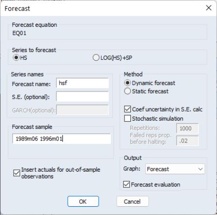
If you press the button, EViews will open a dialog prompting you for your forecast specification.
The resulting dialog is a slightly more complex version of the basic dialog, providing you with a new section allowing you to choose between two series to forecast: the normalized series, HS, or the equation dependent variable, LOG(HS)+SP.
Simply select the radio button for the desired forecast series. Note that you are not provided with the opportunity to forecast SP directly since HS, the first series that appears on the left-hand side of the estimation equation, is offered as the choice of normalized series.
It is important to note that the method is available since EViews is able to determine that the forecast equation has dynamic elements, with HS appearing on the left-hand side of the equation (either directly as HS or in the expression LOG(HS)+SP) and on the right-hand side of the equation in lagged form. If you select dynamic forecasting, previously forecasted values for HS(-1) will be used in forming forecasts of either HS or LOG(HS)+SP.
If the formula can be normalized, EViews will compute the forecasts of the transformed dependent variable by first forecasting the normalized series and then transforming the forecasts of the normalized series. This methodology has important consequences when the formula includes lagged series. For example, consider the following two models:
series dhs = d(hs)
equation eq1.ls d(hs) c sp
equation eq2.ls dhs c sp
The dynamic forecasts of the first difference D(HS) from the first equation will be numerically identical to those for DHS from the second equation. However, the static forecasts for D(HS) from the two equations will not be identical. In the first equation, EViews knows that the dependent variable is a transformation of HS, so it will use the actual lagged value of HS in computing the static forecast of the first difference D(HS). In the second equation, EViews simply views DY as an ordinary series, so that only the estimated constant and SP are used to compute the static forecast.
One additional word of caution–when you have dependent variables that use lagged values of a series, you should avoid referring to the lagged series before the current series in a dependent variable expression. For example, consider the two equation specifications:
d(hs) c sp
(-hs(-1)+hs) c sp
Both specifications have the first difference of HS as the dependent variable and the estimation results are identical for the two models. However, if you forecast HS from the second model, EViews will try to calculate the forecasts of HS using leads of the actual series HS. These forecasts of HS will differ from those produced by the first model, which may not be what you expected.
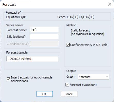
In some cases, EViews will not be able to normalize the dependent variable expression. In this case, the dialog will only offer you the option of forecasting the entire expression. If, for example, you specify your equation as:
log(hs)+1/log(hs) = c(1) + c(2)*hs(-1)
EViews will not be able to normalize the dependent variable for forecasting. The corresponding dialog will reflect this fact.
This version of the dialog only allows you to forecast the dependent variable expression, since EViews is unable to normalize and solve for HS. Note also that only static forecasts are available for this case since EViews is unable to solve for lagged values of HS on the right hand-side.
Plotted Standard Errors
When you select Forecast graph in the forecast dialog, EViews will plot the forecasts, along with plus and minus two standard error bands. When you estimate an equation with an expression for the left-hand side, EViews will plot the standard error bands for either the normalized or the unnormalized expression, depending upon which term you elect to forecast.
If you elect to predict the normalized dependent variable, EViews will automatically account for any nonlinearity in the standard error transformation. The next section provides additional details on the procedure used to normalize the upper and lower error bounds.
Saved Forecast Standard Errors
If you provide a name in this edit box, EViews will store the standard errors of the underlying series or expression that you chose to forecast.
When the dependent variable of the equation is a simple series or an expression involving only linear transformations, the saved standard errors will be exact (except where the forecasts do not account for coefficient uncertainty, as described below). If the dependent variable involves nonlinear transformations, the saved forecast standard errors will be exact if you choose to forecast the entire formula. If you choose to forecast the underlying endogenous series, the forecast uncertainty cannot be computed exactly, and EViews will provide a linear (first-order) approximation to the forecast standard errors.
Consider the following equations involving a formula dependent variable:
d(hs) c sp
log(hs) c sp
For the first equation, you may choose to forecast either HS or D(HS). In both cases, the forecast standard errors will be exact, since the expression involves only linear transformations. The two standard errors will, however, differ in dynamic forecasts since the forecast standard errors for HS take into account the forecast uncertainty from the lagged value of HS. In the second example, the forecast standard errors for LOG(HS) will be exact. If, however, you request a forecast for HS itself, the standard errors saved in the series will be the approximate (linearized) forecast standard errors for HS.
Note that when EViews displays a graph view of the forecasts together with standard error bands, the standard error bands are always exact. Thus, in forecasting the underlying dependent variable in a nonlinear expression, the standard error bands will not be the same as those you would obtain by constructing series using the linearized standard errors saved in the workfile.
Suppose in our second example above that you store the forecast of HS and its standard errors in the workfile as the series HSHAT and SE_HSHAT. Then the approximate two standard error bounds can be generated manually as:
series hshat_high1 = hshat + 2*se_hshat
series hshat_low1 = hshat - 2*se_hshat
These forecast error bounds will be symmetric about the point forecasts HSHAT.
On the other hand, when EViews plots the forecast error bounds of HS, it proceeds in two steps. It first obtains the forecast of LOG(HS) and its standard errors (named, say, LHSHAT and SE_LHSHAT) and forms the forecast error bounds on LOG(HS):
lhshat + 2*se_lhshat
lhshat - 2*se_lhshat
It then normalizes (inverts the transformation) of the two standard error bounds to obtain the prediction interval for HS:
series hshat_high2 = exp(hshat + 2*se_hshat)
series hshat_low2 = exp(hshat - 2*se_hshat)
Because this transformation is a non-linear transformation, these bands will not be symmetric around the forecast.
To take a more complicated example, suppose that you generate the series DLHS and LHS, and then estimate three equivalent models:
series dlhs = dlog(hs)
series lhs = log(hs)
equation eq1.ls dlog(hs) c sp
equation eq2.ls d(lhs) c sp
equation eq3.ls dlhs c sp
The estimated equations from the three models are numerically identical. If you choose to forecast the underlying dependent (normalized) series from each model, EQ1 will forecast HS, EQ2 will forecast LHS (the log of HS), and EQ3 will forecast DLHS (the first difference of the logs of HS, LOG(HS)–LOG(HS(–1)). The forecast standard errors saved from EQ1 will be linearized approximations to the forecast standard error of HS, while those from the latter two will be exact for the forecast standard error of LOG(HS) and the first difference of the logs of HS.
Static forecasts from all three models are identical because the forecasts from previous periods are not used in calculating this period's forecast when performing static forecasts. For dynamic forecasts, the log of the forecasts from EQ1 will be identical to those from EQ2 and the log first difference of the forecasts from EQ1 will be identical to the first difference of the forecasts from EQ2 and to the forecasts from EQ3. For static forecasts, the log first difference of the forecasts from EQ1 will be identical to the first difference of the forecasts from EQ2. However, these forecasts differ from those obtained from EQ3 because EViews does not know that the generated series DLY is actually a difference term so that it does not use the dynamic relation in the forecasts.
Forecasting with Auto-updating series
When forecasting from an equation that contains auto-updating series defined by formulae, the central question is whether EViews interprets the series as ordinary series, or whether it treats the auto-updating series as expressions.
Suppose for example, that we have defined auto-updating series LOGHS and LOGHSLAG, for the log of HAS and the log of HS(-1), respectively,
frml loghs = log(hs)
frml loghslag = log(hs(-1))
and that we employ these auto-updating series in estimating an equation specification:
loghs c loghslag
It is worth pointing out this specification yields results that are identical to those obtained from estimating an equation using the expressions directly using LOG(HS) and LOG(HS(-1)):
log(hs) c log(hs(-1))
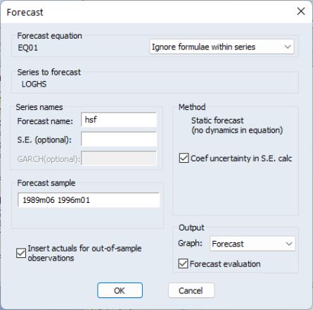
The dialog for the first equation specification (using LOGHS and LOGHSLAG) contains an additional dropdown menu allowing you to specify whether to interpret the auto-updating series as ordinary series, or whether to look inside LOGHS and LOGHSLAG to use their expressions.
By default, the dropdown menu is set to , so that LOGHS and LOGHSLAG are viewed as ordinary series. Note that since EViews ignores the expressions underlying the auto-updating series, you may only forecast the dependent series LOGHS, and there are no dynamics implied by the equation.
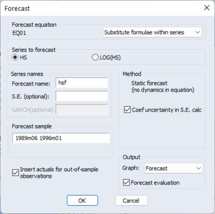
Alternatively, you may instruct EViews to use the expressions in place of all auto-updating series by changing the dropdown menu setting to .
If you elect to substitute the formulae, the dialog will change to reflect the use of the underlying expressions as you may now choose between forecasting HS or LOG(HS). We also see that when you use the substituted expressions you are able to perform either dynamic or static forecasting.
It is worth noting that substituting expressions yields a dialog that offers the same options as if you were to forecast from the second equation specification above—using LOG(HS) as the dependent series expression, and LOG(HS(-1)) as an independent series expression.