Equation Output
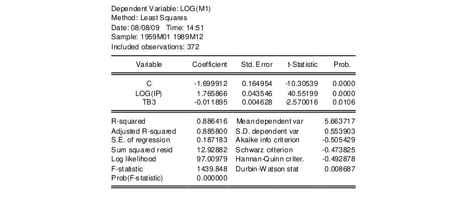
When you click OK in the dialog, EViews displays the equation window displaying the estimation output view (the examples in this chapter are obtained using the workfile “Basics.WF1”):
Using matrix notation, the standard regression may be written as:
 | (20.2) |
where

is a

-dimensional vector containing observations on the dependent variable,

is a

matrix of independent variables,

is a

‑vector of coefficients, and

is a

‑vector of disturbances.

is the number of observations and

is the number of right-hand side regressors.
In the output above,

is log(M1),

consists of three variables C, log(IP), and TB3, where

and

.
Coefficient Results
Regression Coefficients
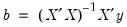
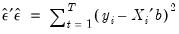
The column labeled “Coefficient” depicts the estimated coefficients. The least squares regression coefficients

are computed by the standard OLS formula:
 | (20.3) |
If your equation is specified by list, the coefficients will be labeled in the “Variable” column with the name of the corresponding regressor; if your equation is specified by formula, EViews lists the actual coefficients, C(1), C(2), etc.
For the simple linear models considered here, the coefficient measures the marginal contribution of the independent variable to the dependent variable, holding all other variables fixed. If you have included “C” in your list of regressors, the corresponding coefficient is the constant or intercept in the regression—it is the base level of the prediction when all of the other independent variables are zero. The other coefficients are interpreted as the slope of the relation between the corresponding independent variable and the dependent variable, assuming all other variables do not change.
Standard Errors
The “Std. Error” column reports the estimated standard errors of the coefficient estimates. The standard errors measure the statistical reliability of the coefficient estimates—the larger the standard errors, the more statistical noise in the estimates. If the errors are normally distributed, there are about 2 chances in 3 that the true regression coefficient lies within one standard error of the reported coefficient, and 95 chances out of 100 that it lies within two standard errors.
The covariance matrix of the estimated coefficients is computed as:
 | (20.4) |
where

is the residual. The standard errors of the estimated coefficients are the square roots of the diagonal elements of the coefficient covariance matrix. You can view the whole covariance matrix by choosing .
t-Statistics
The t-statistic, which is computed as the ratio of an estimated coefficient to its standard error, is used to test the hypothesis that a coefficient is equal to zero. To interpret the t-statistic, you should examine the probability of observing the t-statistic given that the coefficient is equal to zero. This probability computation is described below.
In cases where normality can only hold asymptotically, EViews will often report a z-statistic instead of a t-statistic.
Probability
The last column of the output shows the probability of drawing a t-statistic (or a z-statistic) as extreme as the one actually observed, under the assumption that the errors are normally distributed, or that the estimated coefficients are asymptotically normally distributed.
This probability is also known as the p-value or the marginal significance level. Given a p-value, you can tell at a glance if you reject or accept the hypothesis that the true coefficient is zero against a two-sided alternative that it differs from zero. For example, if you are performing the test at the 5% significance level, a p-value lower than 0.05 is taken as evidence to reject the null hypothesis of a zero coefficient. If you want to conduct a one-sided test, the appropriate probability is one-half that reported by EViews.
For the above example output, the hypothesis that the coefficient on TB3 is zero is rejected at the 5% significance level but not at the 1% level. However, if theory suggests that the coefficient on TB3 cannot be positive, then a one-sided test will reject the zero null hypothesis at the 1% level.
The
p-values for
t-statistics are computed from a
t-distribution with

degrees of freedom. The
p-value for
z-statistics are computed using the standard normal distribution.
Summary Statistics
R-squared
The R-squared (

) statistic measures the success of the regression in predicting the values of the dependent variable within the sample. In standard settings,

may be interpreted as the fraction of the variance of the dependent variable explained by the independent variables. The statistic will equal one if the regression fits perfectly, and zero if it fits no better than the simple mean of the dependent variable. It can be negative for a number of reasons. For example, if the regression does not have an intercept or constant, if the regression contains coefficient restrictions, or if the estimation method is two-stage least squares or ARCH.
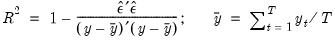
EViews computes the (centered)

as:
 | (20.5) |
where

is the mean of the dependent (left-hand) variable.
Adjusted R-squared
One problem with using

as a measure of goodness of fit is that the

will never decrease as you add more regressors. In the extreme case, you can always obtain an

of one if you include as many independent regressors as there are sample observations.
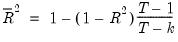
The adjusted

, commonly denoted as

, penalizes the

for the addition of regressors which do not contribute to the explanatory power of the model. The adjusted

is computed as:
 | (20.6) |
The

is never larger than the

, can decrease as you add regressors, and for poorly fitting models, may be negative.
Standard Error of the Regression (S.E. of regression)
The standard error of the regression is a summary measure based on the estimated variance of the residuals. The standard error of the regression is computed as:
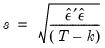 | (20.7) |
Sum-of-Squared Residuals
The sum-of-squared residuals can be used in a variety of statistical calculations, and is presented separately for your convenience:
 | (20.8) |
Log Likelihood
EViews reports the value of the log likelihood function (assuming normally distributed errors) evaluated at the estimated values of the coefficients. Likelihood ratio tests may be conducted by looking at the difference between the log likelihood values of the restricted and unrestricted versions of an equation.
The log likelihood is computed as:
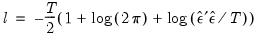 | (20.9) |
When comparing EViews output to that reported from other sources, note that EViews does not ignore constant terms in the log likelihood.
Durbin-Watson Statistic
The Durbin-Watson statistic measures the serial correlation in the residuals. The statistic is computed as
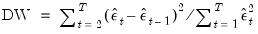 | (20.10) |
See Johnston and DiNardo (1997, Table D.5) for a table of the significance points of the distribution of the Durbin-Watson statistic.
As a rule of thumb, if the DW is less than 2, there is evidence of positive serial correlation. The DW statistic in our output is very close to one, indicating the presence of serial correlation in the residuals. See
“Background”, for a more extensive discussion of the Durbin-Watson statistic and the consequences of serially correlated residuals.
There are better tests for serial correlation. In
“Testing for Serial Correlation”, we discuss the
Q-statistic, and the Breusch-Godfrey LM test, both of which provide a more general testing framework than the Durbin-Watson test.
Mean and Standard Deviation (S.D.) of the Dependent Variable
The mean and standard deviation of

are computed using the standard formulae:
 | (20.11) |
Akaike Information Criterion
The Akaike Information Criterion (AIC) is computed as:
 | (20.12) |
where

is the log likelihood (given by
Equation (20.9)).
The AIC is often used in model selection for non-nested alternatives—smaller values of the AIC are preferred. For example, you can choose the length of a lag distribution by choosing the specification with the lowest value of the AIC. See
Appendix E. “Information Criteria”, for additional discussion.
Schwarz Criterion
The Schwarz Criterion (SC) is an alternative to the AIC that imposes a larger penalty for additional coefficients:
 | (20.13) |
Hannan-Quinn Criterion
The Hannan-Quinn Criterion (HQ) employs yet another penalty function:
 | (20.14) |
F-Statistic
The F-statistic reported in the regression output is from a test of the hypothesis that all of the slope coefficients (excluding the constant, or intercept) in a regression are zero. For ordinary least squares models, the F-statistic is computed as:
 | (20.15) |
Under the null hypothesis with normally distributed errors, this statistic has an
F-distribution with

numerator degrees of freedom and

denominator degrees of freedom.
The p-value given just below the F-statistic, denoted Prob(F-statistic), is the marginal significance level of the F-test. If the p-value is less than the significance level you are testing, say 0.05, you reject the null hypothesis that all slope coefficients are equal to zero. For the example above, the p-value is essentially zero, so we reject the null hypothesis that all of the regression coefficients are zero. Note that the F-test is a joint test so that even if all the t-statistics are insignificant, the F-statistic can be highly significant.
Note that since the
F-statistic depends only on the sums-of-squared residuals of the estimated equation, it is not robust to heterogeneity or serial correlation. The use of robust estimators of the coefficient covariances (
“Robust Standard Errors”) will have no effect on the
F-statistic. If you do choose to employ robust covariance estimators, EViews will also report a robust Wald test statistic and
p-value for the hypothesis that all non-intercept coefficients are equal to zero.
Working With Equation Statistics
The regression statistics reported in the estimation output view are stored with the equation. These equation data members are accessible through special “@-functions”. You can retrieve any of these statistics for further analysis by using these functions in genr, scalar, or matrix expressions. If a particular statistic is not computed for a given estimation method, the function will return an NA.
There are three kinds of “@-functions”: those that return a scalar value, those that return matrices or vectors, and those that return strings.
Selected Keywords that Return Scalar Values
@aic | Akaike information criterion |
@coefcov(i,j) | covariance of coefficient estimates  and  |
@coefs(i) | i-th coefficient value |
@dw | Durbin-Watson statistic |
@f | F-statistic |
@fprob | F-statistic probability. |
@hq | Hannan-Quinn information criterion |
@jstat | J-statistic — value of the GMM objective function (for GMM) |
@logl | value of the log likelihood function |
@meandep | mean of the dependent variable |
@ncoef | number of estimated coefficients |
@r2 | R-squared statistic |
@rbar2 | adjusted R-squared statistic |
@rlogl | retricted (constant only) log-likelihood. |
@regobs | number of observations in regression |
@schwarz | Schwarz information criterion |
@sddep | standard deviation of the dependent variable |
@se | standard error of the regression |
@ssr | sum of squared residuals |
@stderrs(i) | standard error for coefficient  |
@tstats(i) | t-statistic value for coefficient  |
c(i) | i-th element of default coefficient vector for equation (if applicable) |
Selected Keywords that Return Vector or Matrix Objects
@coefcov | matrix containing the coefficient covariance matrix |
@coefs | vector of coefficient values |
@stderrs | vector of standard errors for the coefficients |
@tstats | vector of t-statistic values for coefficients |
@pvals | vector of p-values for coefficients |
Selected Keywords that Return Strings
@command | full command line form of the estimation command |
@smpl | description of the sample used for estimation |
@updatetime | string representation of the time and date at which the equation was estimated |
See also
“Equation” for a complete list.
Functions that return a vector or matrix object should be assigned to the corresponding object type. For example, you should assign the results from @tstats to a vector:
vector tstats = eq1.@tstats
and the covariance matrix to a matrix:
matrix mycov = eq1.@cov
You can also access individual elements of these statistics:
scalar pvalue = 1-@cnorm(@abs(eq1.@tstats(4)))
scalar var1 = eq1.@covariance(1,1)
For documentation on using vectors and matrices in EViews, see
“Matrix Language”.