Nonlinear Least Squares
Suppose that we have the regression specification:
 | (21.28) |
where

is a general function of the explanatory variables

and the parameters

. Least squares estimation chooses the parameter values that minimize the sum of squared residuals:
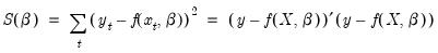 | (21.29) |
We say that a model is
linear in parameters if the derivatives of

with respect to the parameters do not depend upon

; if the derivatives are functions of

, we say that the model is
nonlinear in parameters.
For example, consider the model given by:
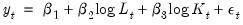 | (21.30) |
It is easy to see that this model is linear in its parameters, implying that it can be estimated using ordinary least squares.
In contrast, the equation specification:
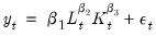 | (21.31) |
has derivatives that depend upon the elements of

. There is no way to rearrange the terms in this model so that ordinary least squares can be used to minimize the sum-of-squared residuals. We must use nonlinear least squares techniques to estimate the parameters of the model.
Nonlinear least squares minimizes the sum-of-squared residuals with respect to the choice of parameters

. While there is no closed form solution for the parameters, estimates my be obtained from iterative methods as described in
“Optimization Algorithms”.
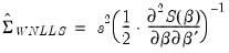
Estimates of the coefficient covariance take the general form:
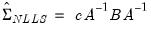 | (21.32) |
where

is an estimate of the information,

is the variance of the residual weighted gradients, and

is a scale parameter.
For the ordinary covariance estimator, we assume that

. Then we have
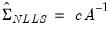 | (21.33) |
where

is an estimator of the residual variance (with or without degree-of-freedom correction).
As in Amemiya (1983), we may estimate

using the outer-product of the gradients (OPG) so we have
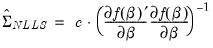 | (21.34) |
where the derivatives are evaluated at

.
Similarly, we may set

to the one-half of the Hessian matrix of second derivatives of the sum-of-squares function:
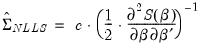 | (21.35) |
evaluated at

.
Alternately, we may assume distinct

and

and employ a White or HAC sandwich estimator for the coefficient covariance as in
“Robust Standard Errors”. In this case,

is estimated using the OPG or Hessian, and the

is a robust estimate of the variance of the gradient weighted residuals. In this case,

is a scalar representing the degree-of-freedom correction, if employed.
For additional discussion of nonlinear estimation, see Pindyck and Rubinfeld (1998, p. 265-273), Davidson and MacKinnon (1993), or Amemiya(1983).
Estimating NLS Models in EViews
It is easy to tell EViews that you wish to estimate the parameters of a model using nonlinear least squares. EViews automatically applies nonlinear least squares to any regression equation that is nonlinear in its coefficients. Simply select , enter the equation in the equation specification dialog box, and click OK. EViews will do all of the work of estimating your model using an iterative algorithm.
A full technical discussion of iterative estimation procedures is provided in
Appendix C. “Estimation and Solution Options”.
Specifying Nonlinear Least Squares
For nonlinear regression models, you will have to enter your specification in equation form using EViews expressions that contain direct references to coefficients. You may use elements of the default coefficient vector C (e.g. C(1), C(2), C(34), C(87)), or you can define and use other coefficient vectors. For example:
y = c(1) + c(2)*(k^c(3)+l^c(4))
is a nonlinear specification that uses the first through the fourth elements of the default coefficient vector, C.
To create a new coefficient vector, select in the main menu and provide a name. You may now use this coefficient vector in your specification. For example, if you create a coefficient vector named CF, you can rewrite the specification above as:
y = cf(11) + cf(12)*(k^cf(13)+l^cf(14))
which uses the eleventh through the fourteenth elements of CF.
You can also use multiple coefficient vectors in your specification:
y = c(11) + c(12)*(k^cf(1)+l^cf(2))
which uses both C and CF in the specification.
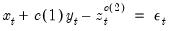
It is worth noting that EViews implicitly adds an additive disturbance to your specification. For example, the input
y = (c(1)*x + c(2)*z + 4)^2
is interpreted as
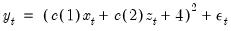
, and EViews will minimize:
 | (21.36) |
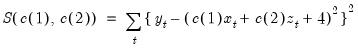
If you wish, the equation specification may be given by a simple expression that does not include a dependent variable. For example, the input,
(c(1)*x + c(2)*z + 4)^2
is interpreted by EViews as
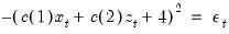
, and EViews will minimize:
 | (21.37) |
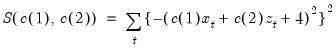
While EViews will estimate the parameters of this last specification, the equation cannot be used for forecasting and cannot be included in a model. This restriction also holds for any equation that includes coefficients to the left of the equal sign. For example, if you specify,
x + c(1)*y = z^c(2)
EViews will find the values of C(1) and C(2) that minimize the sum of squares of the implicit equation:
 | (21.38) |
The estimated equation cannot be used in forecasting or included in a model, since there is no dependent variable.
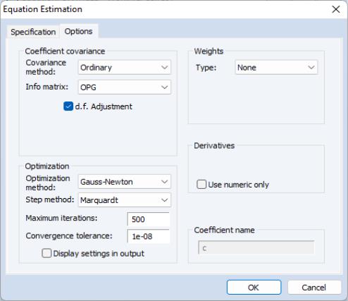
Estimation Options
Clicking on the tab displays the nonlinear least squares estimation options:
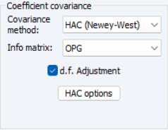
Coefficient Covariance
EViews allows you to compute ordinary coefficient covariances using the inverse of either the OPG of the mean function or the observed Hessian of the objective function, or to compute robust sandwich estimators for the covariance matrix using White or HAC (Newey-West) estimators.
• The topmost dropdown menu should be used to choose between the default or the robust or methods.
• In the menu you should choose between the and the estimators for the information.
• If you select , you will be presented with a button that, if pressed, brings up a dialog to allow you to control the long-run variance computation.
See
“Robust Standard Errors” for a discussion of White and HAC standard errors.
You may use the checkbox to enable or disable the degree-of-freedom correction for the coefficient covariance. For the method, this setting amounts to determining whether the residual variance estimator is or is not degree-of-freedom corrected. For the sandwich estimators, the degree-of-freedom correction is applied to the entire matrix.
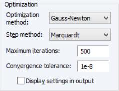
Optimization
You may control the iterative process by specifying the optimization method, convergence criterion, and maximum number of iterations.
The dropdown menu lets you choose between the default and , , and methods.
In general, the differences between the estimates should be small for well-behaved nonlinear specifications, but if you are experiencing trouble, you may wish to experiment with methods. Note that EViews legacy is a particular implementation of Gauss-Newton with Marquardt or line search steps, and is provided for backward estimation compatibility.
The menu allows you to select the approach for candidate iterative steps. The default method is , but you may instead select or .
EViews will report that the estimation procedure has converged if the convergence test value is below your convergence tolerance. While there is no best choice of convergence tolerance, and the choice is somewhat individual, as a guideline note that we generally set ours something on the order of 1e‑8 or so and then adjust it upward if necessary for models with difficult to compute numeric derivatives.
See
“Iteration and Convergence” for additional discussion.
In most cases, you need not change the maximum number of iterations. However, for some difficult to estimate models, the iterative procedure may not converge within the maximum number of iterations. If your model does not converge within the allotted number of iterations, one solution is to click the button and increase the maximum number of iterations. Click to accept the options, and OK again to begin estimation. EViews will start estimation using the last set of parameter values as starting values.
These options may also be set from the global options dialog. See
Appendix A,
“Estimation Defaults” for details.
Derivative Methods
Estimation in EViews requires computation of the derivatives of the regression function with respect to the parameters.
In most cases, you need not worry about the settings for the derivative computation. The EViews estimation engine will employ analytic expressions for the derivatives, if possible, or will compute high numeric derivatives, switching between lower precision computation early in the iterative procedure and higher precision computation for later iterations and final computation. You may elect to use only numeric derivatives.
See
“Derivative Computation” for additional discussion.
Starting Values
Iterative estimation procedures require starting values for the coefficients of the model. The closer to the true values the better, so if you have reasonable guesses for parameter values, these can be useful. In some cases, you can obtain good starting values by estimating a restricted version of the model using least squares. In general, however, you may need to experiment in order to find starting values.
There are no general rules for selecting starting values for parameters so there are no settings in this page for choosing values. EViews uses the values in the coefficient vector at the time you begin the estimation procedure as starting values for the iterative procedure. It is easy to examine and change these coefficient starting values. To see the current starting values, double click on the coefficient vector in the workfile directory. If the values appear to be reasonable, you can close the window and proceed with estimating your model.
If you wish to change the starting values, first make certain that the spreadsheet view of your coefficients is in edit mode, then enter the coefficient values. When you are finished setting the initial values, close the coefficient vector window and estimate your model.
You may also set starting coefficient values from the command window using the PARAM command. Simply enter the PARAM keyword, followed by each coefficient and desired value. For example, if your default coefficient vector is C, the statement:
param c(1) 153 c(2) .68 c(3) .15
sets C(1)=153, C(2)=.68, and C(3)=.15.
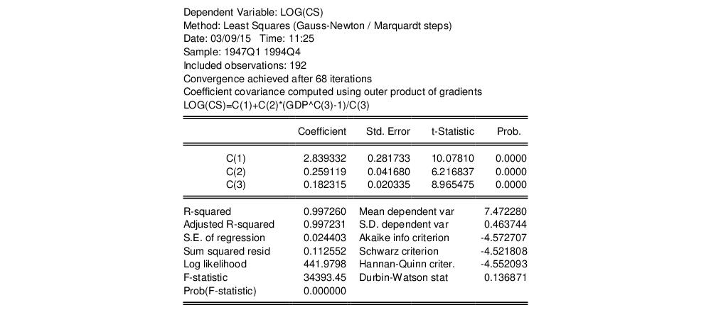
Output from NLS
Once your model has been estimated, EViews displays an equation output screen showing the results of the nonlinear least squares procedure. Below is the output from a regression of LOG(CS) on C, and the Box-Cox transform of GDP using the data in the workfile “Chow_var.WF1”:
If the estimation procedure has converged, EViews will report this fact, along with the number of iterations that were required. If the iterative procedure did not converge, EViews will report “Convergence not achieved after” followed by the number of iterations attempted.
Below the line describing convergence, and a description of the method employed in computing the coefficient covariances, EViews will repeat the nonlinear specification so that you can easily interpret the estimated coefficients of your model.
EViews provides you with all of the usual summary statistics for regression models. Provided that your model has converged, the standard statistical results and tests are asymptotically valid.
NLS with ARMA errors
EViews will estimate nonlinear regression models with autoregressive error terms. Simply select or and specify your model using EViews expressions, followed by an additive term describing the AR correction enclosed in square brackets. The AR term should consist of a coefficient assignment for each AR term, separated by commas. For example, if you wish to estimate,
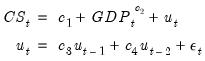 | (21.39) |
you should enter the specification:
cs = c(1) + gdp^c(2) + [ar(1)=c(3), ar(2)=c(4)]
See “Initializing the AR Errors” for additional details. EViews does not currently estimate nonlinear models with MA errors, nor does it estimate weighted models with AR terms—if you add AR terms to a weighted nonlinear model, the weighting series will be ignored.
Weighted NLS
Weights can be used in nonlinear estimation in a manner analogous to weighted linear least squares in equations without ARMA terms. To estimate an equation using weighted nonlinear least squares, enter your specification, press the button and fill in the weight specification.
EViews minimizes the sum of the weighted squared residuals:
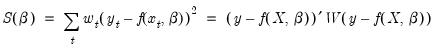 | (21.40) |
with respect to the parameters

, where

are the values of the weight series and

is the diagonal matrix of weights. The first-order conditions are given by,
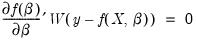 | (21.41) |
and the default OPG d.f. corrected covariance estimate is computed as:
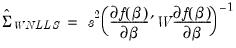 | (21.42) |
and the corresponding Hessian estimate is
 | (21.43) |
for the weighted objective function given in
Equation (21.41).
One may elect, of course, to compute a White or HAC sandwich estimator for the coefficient covariance as in
“Robust Standard Errors”.
Solving Estimation Problems
EViews may not be able to estimate your nonlinear equation on the first attempt. Sometimes, the nonlinear least squares procedure will stop immediately. Other times, EViews may stop estimation after several iterations without achieving convergence. EViews might even report that it cannot improve the sums-of-squares. While there are no specific rules on how to proceed if you encounter these estimation problems, there are a few general areas you might want to examine.
Starting Values
If you experience problems with the very first iteration of a nonlinear procedure, the problem is almost certainly related to starting values. See the discussion in
“Starting Values” for details on how to examine and change your starting values.
Model Identification
If EViews goes through a number of iterations and then reports that it encounters a “Near Singular Matrix”, you should check to make certain that your model is identified. Models are said to be non-identified if there are multiple sets of coefficients which identically yield the minimized sum-of-squares value. If this condition holds, it is impossible to choose between the coefficients on the basis of the minimum sum-of-squares criterion.
For example, the nonlinear specification:
 | (21.44) |
is not identified, since any coefficient pair

is indistinguishable from the pair

in terms of the sum-of-squared residuals.
For a thorough discussion of identification of nonlinear least squares models, see Davidson and MacKinnon (1993, Sections 2.3, 5.2 and 6.3).
Optimization Algorithm
In general, the choice of optimization algorithm should have little effect on the computation of estimates. That said, if you are experiencing trouble, you may wish to experiment with different methods. In addition, you may wish to experiment with different optimizers to ensure that your estimates are robust to the choice of optimization method.
Note that EViews legacy is a particular implementation of Gauss-Newton with Marquardt or line search steps, and is provided for backward estimation compatibility.
See
“Optimization” for discussion.
Convergence Criterion
EViews may report that it is unable to improve the sums-of-squares. This result may be evidence of non-identification or model misspecification. Alternatively, it may be the result of setting your convergence criterion too low, which can occur if your nonlinear specification is particularly complex.
If you wish to change the convergence criterion, enter the new value in the tab. Be aware that increasing this value increases the possibility that you will stop at a local minimum, and may hide misspecification or non-identification of your model.
See
“Setting Estimation Options”, for related discussion.