Technical Discussion
Impulse Response Standard Errors and Confidence Intervals
Traditionally, confidence intervals for VAR impulse responses have been based on the Lütkepohl (1990) asymptotic approximation and EViews provides these values for ordinary VAR estimators. Nevertheless, it is well known that asymptotic validity is often questionable in small samples. In this regard, Monte Carlo and bootstrap methods are of considerable practical interest as they often perform better when the number of observations is limit
The VAR Bootstrap
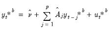
To formalize matters, consider a system of time series of length T. If the system is modelled as a vector autoregression (VAR) process of order p, the data generating process (DGP) for the system is written as:
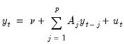 | (44.38) |
where

and

are

-element vectors,

are

matrices, and
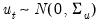
where

is a

covariance matrix.
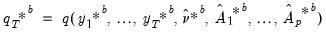
Next suppose that the object of interest (e.g., estimator, test statistic, etc.) is the functional:
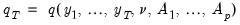 | (44.39) |
The distribution

of

may be approximated by generating a large number, say
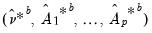
B, of different outcome paths (

for

) for the “*” is used to indicate that the object is derived from simulation. In particular, the
B outcomes

are obtained by simulating from the DGP in
Equation (44.38) to generate
B independent outcomes

of

and for each such draw, compute the corresponding

using
Equation (44.39) but with the generated data. The distribution of the

is then estimated as the empirical distribution of the set of simulated outcomes

.
There are a variety of simulating data from the DGP. EViews supports three: residual based bootstrap, residual based double bootstrap, fast double bootstrap. We consider each in turn.
Residual Based Bootstrap
A commonly used method of generating data from
Equation (44.38) is the
residual based bootstrap. The procedure is straightforward:
1. Using the original data

and the specification
Equation (44.38), obtain estimates of the coefficients
and the corresponding the residual series

.
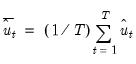
2. Derive the centered residual series

, where

.
3. For each

:
• Draw a series of length
T of bootstrap innovations

by randomly drawing with replacement from the

.
• Generate a bootstrap DGP of

as follows:
 | (44.40) |
• Using the generated

, estimate coefficients to obtain

.
• Obtain a bootstrap estimate of the object of interest
 | (44.41) |
4. The final bootstrap estimator of

, typically denoted as

is obtained as the average of the individual bootstrap estimates

. In other words
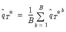 | (44.42) |
Residual Based Double Bootstrap
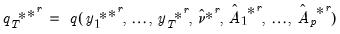
It is sometimes necessary to obtain bootstrap statistics of a bootstrap statistic, for example, when the object of interest is the distribution

of the

-th bootstrap estimate

. This distribution is typically needed in deriving the variance of a bootstrap statistics.
In this case, for each

, the distribution

is approximated by generating a large number, say
R, of different outcome paths (

for

), where the superscript “**” indicates that the object is derived from a second stage bootstrap simulation.
In particular, the
R outcomes

are obtained by simulating, from the bootstrap DGP, using a bootstrap draw of
b and
Equation (44.40) and generating new
R outcomes

and then for each of those outcomes, a corresponding

. The distribution of the

is then estimated as the empirical distribution of the set of simulated outcomes

.
The resampling procedure used to derive these second stage bootstrap statistics is the residual bootstrap double bootstrap. The algorithm is summarized below:
1. Using the original data

and the specification
Equation (44.38), obtain estimates of the coefficients

and the corresponding the residual series

.
2. Derive the centered residual series

, where
.
3. For each

:
• Perform a residual bootstrap: draw bootstrap residuals

from the

, generate bootstrap data

, estimate
, and obtain the first stage bootstrap estimate
 | (44.43) |
This step is the same as each step in the standard residual bootstrap.
• Derive first stage bootstrap residuals based on the bootstrap data
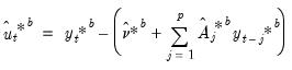 | (44.44) |
and obtain centered first stage bootstrap residuals by subtracting off means,
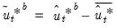 | (44.45) |
where
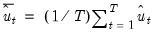
.
• For each

perform a residual bootstrap: draw bootstrap residuals

from the

, generate bootstrap data

, estimate
, and obtain a second stage bootstrap estimate
 | (44.46) |
Fast Double Bootstrap
Performing a full double bootstrap algorithm is extremely computationally demanding. A single bootstrap algorithm typically requires the computation of

test statistics —a single statistic performed on the original data and an additional
B statistics obtained in the bootstrap loop. On the other hand, a full double bootstrap requires

statistics, with the additional BR statistics computed in the inner loop of the double bootstrap algorithm. For instance, setting

and

, the double bootstrap will require the computation of no less than 499,501 test statistics. In this regard, several attempts have been proposed to circumvent this computational burden, among the most popular of which is the fast double bootstrap (FDB) algorithm of Davidson and MacKinnon (2002) and general iterated variants proposed in Davidson and Trokic (2020). The principle governing the success of these algorithms relies on setting

. For instance, the FDB has proved particularly useful in approximating full double bootstrap algorithms with roughly less than the twice the computational burden of the traditional bootstrap:

to be precise.
Bootstrapping Impulse Responses
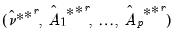
Let

represent an impulse response coefficient that depends on the data. In terms of the discussion above we may think of

and contemplate obtaining bootstrap measures of the precision of

.
VAR Impulse Responses
To derive bootstrap confidence intervals for impulse responses, let

,

, and

denote, respectively, some general impulse response coefficient, its estimator derived using the original data

and the DGP in
Equation (44.38), and the associated bootstrap estimator derived using a procedure like the residual based bootstrap
“Residual Based Bootstrap”.
Next, let denote a given significance level so that the confidence interval of interest has coverage

. Then, the following bootstrap confidence intervals have been considered in the literature. See also Lütkepohl (2005) for further details.
Standard Percentile Confidence Interval
The most common bootstrap algorithm for impulse response CIs is based on the percentile confidence interval described in Efron and Tibshirani (1993). The bootstrap CI is derived as:
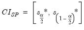 | (44.47) |
where

and

are the

and

quantiles of the empirical distribution of

, respectively.
Hall’s Percentile Confidence Interval
An alternative to the standard percentile CI is the Hall (1992) confidence interval. The idea behind this method is that the distribution of

is asymptotically approximated by the distribution of

. Accordingly, the Hall bootstrap CI is given by
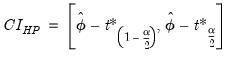 | (44.48) |
where

and

are the

and

quantiles of the empirical distribution of the bootstrap draws
 | (44.49) |
See Hall (1986) for details.
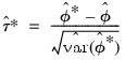
Hall’s Studentized Confidence Interval
Another possible approach to computing the CI is to approximate the distribution of the studentized statistic

,
 | (44.50) |
with the distribution of the bootstrap studentized statistic:
 | (44.51) |
In this case, the bootstrap CI is derived as:
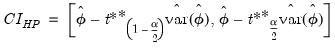 | (44.52) |
where

and

are the

and

quantiles of the empirical distribution of

, where
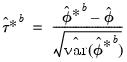 | (44.53) |
See Hall (1986) for details.
Note that

can be obtained from the empirical variance of the
B bootstrap estimates

and that ,

may be estimated from the empirical variance of the
R double bootstrap estimates

.
Clearly, the computations above require a full double bootstrap. An alternative is to use the significantly less computationally demanding fast double bootstrap (FDB) approximation. In this regard, Davidson and Trokic (2020) offer an algorithm that relies on the inverse relationship between
p-values and confidence intervals and only requires

double bootstrap evaluations to compute empirical quantiles.
While the FDB is computationally appealing, care should be taken with its use as Chang and Hall (2015) show that the FDB does not improve asymptotically on the single bootstrap for the construction of confidence intervals.
Killian’s Unbiased Confidence Interval
The Kilian (1998) confidence intervals are specifically designed for VAR impulse response estimates. In particular, this approach explicitly corrects for the bias and skewness in the impulse response estimator that arises due to insufficient observations.
We skip over most of the details of the Kilian computation. Roughly, however, the procedure involves:
• Estimating a VAR to obtain coefficients and then running a residual bootstrap to obtain bootstrap coefficient estimates which are used to compute a bias correction adjustment to the original estimates.
• Using the bias corrected coefficients as the basis of a residual double bootstrap to bias correct each of the bootstrap coefficients.
• Constructing the impulse responses using the bias corrected bootstrap coefficients.
• Deriving the

and

empirical quantiles of the bias corrected bootstrap impulse responses.
Note that the nested bootstrap computations required for this method can be costly. A fast bootstrap approximation may be obtained by computing the bias adjustments only once per loop and using it across replications.
VEC Impulse Responses
The principles governing the computation of bootstrap CIs for VAR impulse responses remain valid for VEC impulse responses as well. Since every VAR(

) has an equivalent representation as a VEC(

) process, one can simply convert bootstrap VAR estimates into their VEC equivalents, and proceed analogously to derive the VEC impulse responses using the latter coefficients. Alternatively, one can start from a VEC representation, obtain bootstrap coefficient estimates, and then integrate the VEC model to its VAR equivalent. The converted bootstrap coefficient estimates can then be used to derive bootstrap CIs for the corresponding VAR.