Estimating ARDL Models in EViews
While linear and nonlinear ARDL models can in fact be estimated using general tools for least squares (or quantile regression in the case of QARDL variants), EViews offers a native interface for estimation.
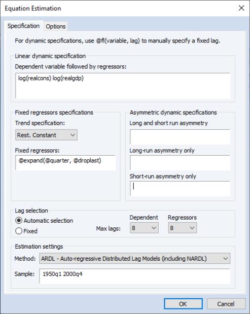
From the main EViews menu, click on Quick/Estimate Equation... to open the equation dialog or click on Object/New Object..., then select Equation and click on the Estimate button. Once the equation dialog opens, select ARDL - Autoregressive Distributed Lag Models from the Method dropdown,
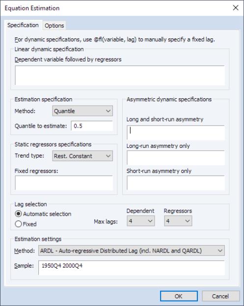
The dialog defaults to the classical ARDL estimation framework, namely least squares. If you prefer to change the estimation method quantile estimation, you may select Quantile from the Method dropdown in the Estimation specification group.
Under the Linear dynamic specification, specify the dependent variable followed by symmetric (distributed-lag) regressors, starting with the dependent (autoregressive) variable,
Next, specify any asymmetric regressors can be specified in the Asymmetric dynamic specifications.
• The Long-run and short-run edit field should be used to specify regressors which are asymmetric in both the long-run and short-run.
• The the Long-run only and the Short-run only edit field should include only asymmetric regressors that are exclusively long-run and short-run, respectively.
For both symmetric and asymmetric dynamic regressors you may specify either the series name and expression, or you may use an
@fl function to specify a regressor and an individual fixed lag

. The syntax of the function is
@fl(variable, lag)
where variable is the series name or expression, and lag is an integer for the fixed lag. An individual fixed lag specified using @fl takes precedence over the overall automatic or fixed lag selection methods specified in the section.
You should specify any exogenous and deterministic regressors in the
Fixed regressors specifications section. The five deterministic cases involving a constant and trend discussed in relation to bounds testing (
“Bounds Test View”), may be specified using the
Trend specification dropdown. Any remaining exogenous regressors should can be specified under the
Fixed regressors edit field.
The section contains settings for the choice of the dependent variable lags

and regressor lags

:
• If you select , EViews will automatically select values for the lags. Following the suggestion of Pesaran, Shin, and Smith (PSS 2001), the lag structure is chosen using standard model selection criteria. You will be prompted to enter a for the variables and .
Select the maximum number of lags to be considered for the dependent and distributed-lag variables by adjusting the
Max lags drop downs for variables and . The total number of models that are evaluated under such procedures is the maximum number of combinations of the set of numbers

and

additional sets of numbers

, so that we have

– where

and
are respectively the maximum number of lags of the dependent and explanatory variables specified at the time of estimation, and
is the total number of distributed-lag regressors. For instance, with 2 distributed-lag regressors and the default values

, the total number of models under consideration would be 100.
Note that EViews offers several model selection procedures including Akaike (AIC), Schwarz (BIC), Hannan-Quinn (HQ), or the adjusted

. You may choose model selection criterion is used by clicking on the
Options tab and selecting the desired method under the
Model Selection Criteria dropdown menu.
• Alternately, you can instruct EViews to use a fixed lag of your choice. Click on enter the for the variables and . The number of regressor lags will be set to the specified value for all variables.
Options
In the case of standard ARDL models, this options dialog looks like the figure below
For QARDL models, the options tab of the estimation dialog provides options for quantile estimation:
The options are those for standard quantile regression estimation, and are described in
“Estimation Options”.