Estimating a Bayesian VAR in EViews
To estimate a Bayesian VAR in EViews, click on or type var in the command window to bring up the dialog. Select the as the in the radio buttons on the left-hand side of the dialog.
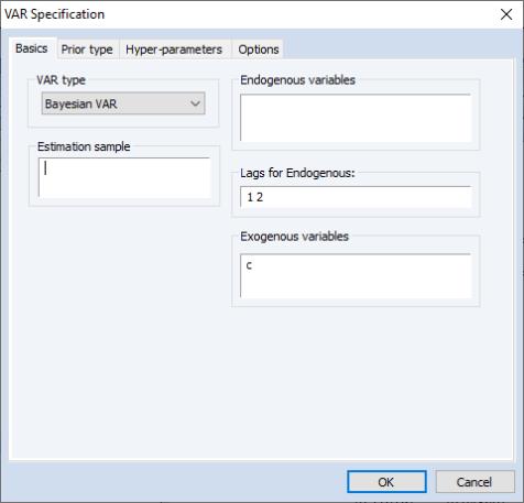
The dialog will change to the BVAR version of the VAR Specification dialog. As with a standard VAR, you may use the page to list of endogenous variables, the included lags, and any exogenous variables, and to specify the estimation sample:
The three BVAR specific tabs—, , and —allow you to customize your specification. The following discussion of the settings on these three tabs assumes that you are familiar with the basics of the various prior types and associated settings. For additional detail, see
“Technical Background”.
Prior Type
The tab lets you specify the type of prior you wish to use, whether to include dummy observations, and options for calculating the initial residual covariance matrix.
You may use the drop-down menu to choose between , , , , , , and priors.
The check boxes allow you to include dummy/additional observations to the data matrices of the VAR. The setting adds observations to account for possible unit-root issues, while the setting adds observations to account for possible cointegration issues (see
“Dummy Observations”).
For the priors other than or n, a dropdown menu allows you to specify how the initial residual covariance matrix is calculated:
• estimates a univariate AR model (with number of lags matching those specified for the VAR) for each endogenous variable, then constructs the residual covariance matrix as a diagonal matrix with diagonal elements equal to the residual variance from the estimated univariate models.
• uses the covariance from an estimated classical VAR model, but zeros out the off-diagonals.
• uses the covariance from an estimated classical VAR model.
• is computed in the same way as the , but only one lag is used.
The radio buttons specify whether to include any exogenous variables specified in the VAR in the calculation of the initial covariance matrix.
• If you select either of the choices, the checkbox specifies whether to include those observations in the initial covariance calculation.
• The selection determines whether to use a degrees-of-freedom correction in the covariance estimate.
If the prior type was selected in the drop-down menu, the checkbox selects whether to use the initial covariances as hyper-parameters, or as the starting values for an optimized hyper-parameter selection.
Finally, the box is used to specify the sample that is used to estimate the covariance. If left blank, the same sample as the overall VAR estimation.
Hyper-parameters
The tab allows specification of the hyper-parameters of the prior distribution.
If the prior type was selected on the tab, the checkbox selects whether to use the values as hyper-parameters, or as the starting values for an optimized hyper-parameter selection.
Note that only hyper-parameters that are available for the current prior type and choice of initial dummy observations are available for selection.
Options
The tab offers options for the Giannone, Lenza & Primiceri (GLP) prior and the inverse normal-Wishart prior. The GLP prior requires optimization of the hyper-parameters, and so options relating to the optimization algorithm; and . The latter requires estimation through a Gibbs Sampler, and so offers options for the number of draws from the sampler, the percentage of draws to discard as burn-in draws, and the random number generator’s seed value.