Examples
Investment Example
To illustrate the Bayesian approach, we first estimate the coefficients of a VAR(2) model using the first differences of the logarithm of the investment (DLINVESTMENT), income (DLINCOME), and consumption (DLCONCUMPTION). The raw data are provided in the EViews workfile “wgmacro.WF1”. This data set was examined by Lütkepohl (2007, page 228).
Click on to open the main VAR specification dialog. In the VAR type box, select and in the box, type:
dlincome dlinvestment dlconsumption
Here, you will see the pre-filled settings including the variable names. You may change the default settings, but for now on, we assume that the default settings are used.
Basic Settings
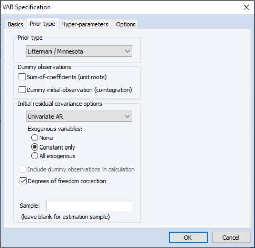
Next, click on the tab to select the prior type for the VAR. By default, EViews will choose the for the and the option for the , but you can change the prior type and the initial covariance calculation option from the menus.
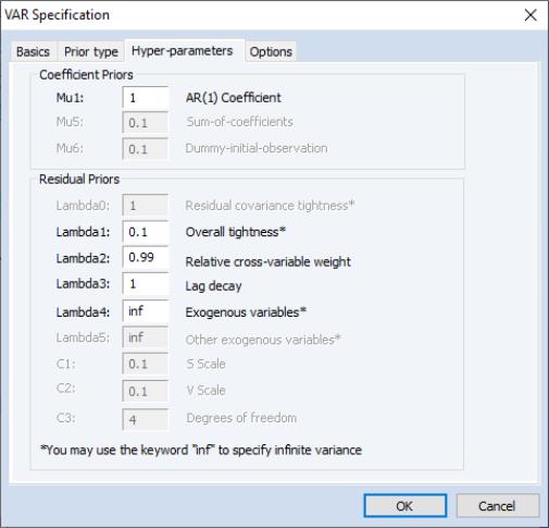
The tab shows the hyper-parameter settings. Note that the settings may vary depending on the prior type. We will only change the hyper-parameter, to be equal to zero (since the data are all differenced):
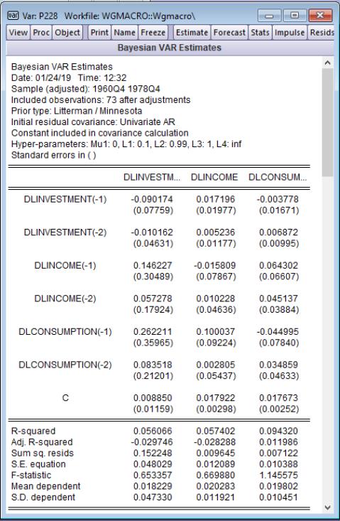
Click on to accept the dialog settings. EViews estimates the VAR and displays the results view. The results are shown below:
The heading information provides the basic information about the settings used in estimation, and the basic prior information, including hyper-parameter values. Just below the heading, the mean and standard errors from the posterior distribution are displayed.
The bottom portion of the output displays standard classical summary statistics for a VAR. Although they do not have a Bayesian interpretation, they are displayed for comparison purposes.
In his study of this data, Lütkepohl chose to use a diagonal VAR to calculate the initial residual covariance. We can replicate his results by setting the Diagonal VAR covariance type on the tab of the dialog:
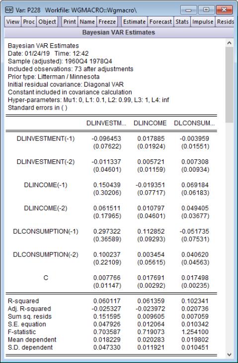
Since the estimates in the third row of Table 5.3 of Lütkepohl’s example may be obtained using EViews’ default hyper-parameter values (other than the previously changed Mu1), click on to estimate the modified BVAR specification:
The results in the other rows of table Table 5.3 may be obtained by changing the hyper-parameters.
Alternate priors
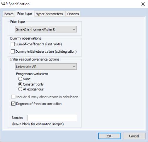
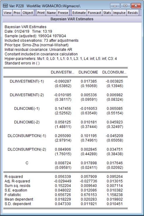
To illustrate the importance of prior selection, we estimate the same model using the Sims-Zha normal-Wishart prior, with the univariate AR calculation for the initial residual covariance, and the default hyper-parameter settings:
We can see that, for these data and VAR specification, changing the prior type did not have a large impact on any of the parameter values:
Macroeconomic Variables Example
As a second example of using Bayesian VARs in EViews, we work with a dataset created by Stock and Watson (2008) which provides data on a number of US macroeconomic variables. The dataset was obtained from Mark Watson’s website:
http://www.princeton.edu/~mwatson/publi.html, and a truncated version, with only variables used in this example, is provided as the EViews workfile “stockwatson.wf1”. These data are used in Giannone, Lenza and Primiceri 2012, among other studies.
We will estimate a VAR using the same series as Giannone, Lenza and Primiceri’s “Medium-scale model”. This model contains seven series: Gross domestic product (GDP), the GDP deflator (GDPI), consumption (CONS), investment (INV), hours worked (HOURS), wages (WAGES), and the federal funds rate (FED). The first six variables were reported at a quarterly frequency. The federal funds rate is reported at a monthly rate, so the quarterly average is used to convert the data to quarterly. All variables have been logged and multiplied by four (to give annualized values), with the exception of the funds rate which is left in levels.
To estimate the VAR we click on to open the main VAR specification dialog. We select as the , and in the box we type:
gdp gdpi cons inv hours wages fed
To estimate the VAR with 5 lags, in the edit field we enter:
1 5
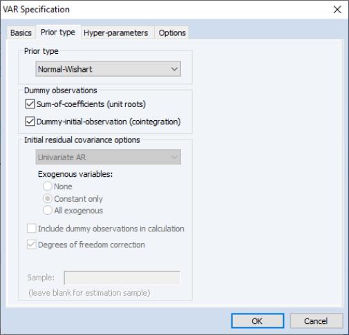
To begin we will estimate with a normal-Wishart prior, including dummy observations to account for both unit roots and cointegration:
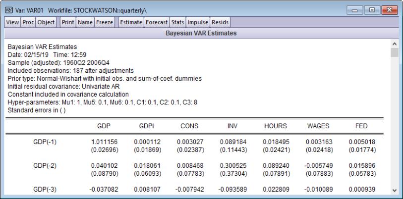
We keep the hyper-parameters at their default values. Clicking will estimate the VAR and display the results (the top portion of which are displayed below):
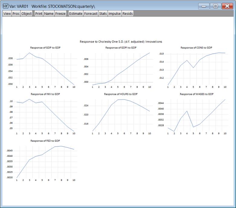
Having estimated the VAR, we will look at the impulse responses to a shock in GDP. We bring up the Impulse Response dialog by clicking the button on the VAR. We enter “GDP” in the box and keep all other settings at their defaults.
Clicking will produce a graph of the responses:
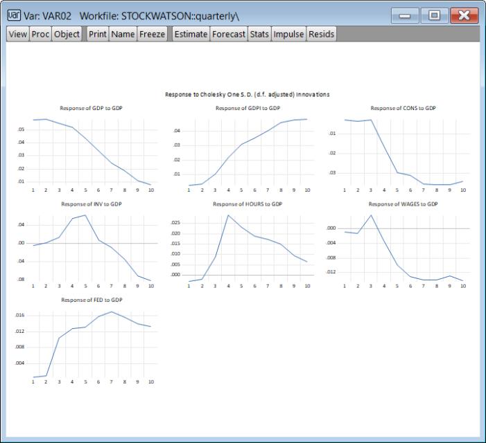
We would like to compare these results with those obtained assuming independent normal-Wishart priors.
We follow the steps above a second time, beginning with estimation, but after changing the prior to . The resulting responses are: