Estimating an Elastic Net Regression in EViews
To estimate an elastic net model, open an existing equation or select from the main EViews menu and select from the main dropdown menu near the bottom of the dialog.
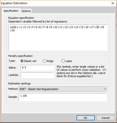
EViews will display a dialog with two tabs: the tab and the tab.
Specification
Focusing first on the page, we see that it has three sections: , , and specification. As the should be familiar, we focus our attention on the first two sections.
Equation Specification
In the section edit field you should enter the dependent variable followed by the regressors. In order to add weights to the variables, use the keyword
@vw() around the variable being weighted, followed by the weight. The weight must be between zero and one and multiplies the

penalty parameter. For example,
@vw(v2, 0) means the variable V2 is not shrunk.
Penalty Specification
Next, in the edit field you should choose from the elastic net, ridge, and Lasso penalties, and enter the desired parameters.
• If you choose the elastic net penalty, EViews will fill in the alpha field with the default value of

, or you may enter a number of your choice. This value must be between zero and one.
• If you choose the ridge penalty, EViews will automatically fill in the alpha field with the ridge parameter

. Note that when ridge regression is chosen, EViews displays the analytic solution.
• If you choose the Lasso penalty, EViews will automatically fill in the alpha field with the Lasso parameter

.
You are free to fill in the lambda field with a single value, multiple values separated by spaces, or a series object from the workfile. If multiple values of lambda are entered, either directly as a list or through a series object, cross-validation will be performed to determine the value giving the model with the lowest measurement error. Note that EViews does not allow multiple values of the

parameter.
You may also leave the lambda field blank. If you choose to do this EViews will generate its own list of values based on the data.
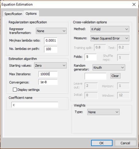
Options
The options dialog allows you specify the data transformation options for the regressors and, potentially, the properties of the lambda path, optimization settings, and details of the cross-validation. Depending of the values of lambda chosen in the window, various options will be available:
• For single values of lambda, the available options will be limited to in the section of the dialog and options in the section. You may choose between (the default), by sample and population, and normalizations, and transformation.
• For multiple supplied values of lambda, the available options will expand to include the . Certain options within this section can be chosen depending on the particular method of cross-validation chosen ( for , for example).
• For multiple EViews-supplied values of lambda (i.e., leaving the text box blank on the window), the remaining options for and will become available. In the text box, supply the ratio of the minimum to the maximum value of lambda desired; the default is 0.0001. In the text box, supply the number of values of lambda on the path; the default is 100.
The portion of the dialog is the same as that used in other estimators such as least squares. For more information, please see
“Weighted Least Squares”.
Cross-validation options
The available cross-validation options include:
• : After the dataset is divided into training and test sets, the ordering is shuffled. The and fields control the details of the shuffling. You may the leave the field blank, in which case EViews will use the clock to obtain a seed at the time of estimation, or you may provide an integer from 0 to 2,147,483,647. The button may be used to clear the seed used by a previously estimated equation. By changing the value of the field from the default of 1 you may create multiple datasets with different, shuffled ordering of training and test sets.
• : The dataset is divided into K evenly spaced “folds” and the ordering is shuffled (the details of the shuffling are determined by the and fields). One fold is held out as the test set while the remaining K-1 folds are combined into the training set. This process is then repeated, with each fold being held out in turn as the test set. After model estimation the statistics are averaged over all K folds.
• : This is the same as K-Fold, but with the number of folds equal to the number of observations.
• : This is similar to K-Fold, with the exception that a test set of size P is held out, with the remaining data forming the training set. This process is repeated over all remaining combinations.
• : After a window size is chosen for the dataset, the window is divided into training and test sets (the default test set size is 1, and you may also choose the test set size as a fraction), with the test set in each window always coming after the training set. The window “rolls” through the dataset until it reaches the end of the dataset. You may also choose how far ahead of the training set you want the test set to be (the horizon), as well as an initial period in the dataset to hold out of the cross-validation (the initial period).
• : The dataset is divided into training and test sets (the default test set size is 1, and only integer test set sizes are allowed), with the test set in each window always coming after the training set. With each iteration the training set size expands by one while the test set stays the same size. You may choose how far ahead of the training set you want the test set to be (the horizon), as well as an initial period in the dataset to hold out of the cross-validation (the initial period).