Examples
We provide some examples of elastic net estimation using the prostate cancer data from Stamey et al, (1989), which also serve as example data in Hastie, Tibshirani, and Friedman (2009, p. 3).
The “Prostate.WF1” workfile containing these data obtained from the authors’ website is provided with your EViews example data.
The dependent variable is the logarithm of prostate-specific antigen (LPSA). The regressors are log(cancer volume) (LCAVOL), log(prostate weight) (LWEIGHT), age, the logarithm of the amount of benign prostatic hyperplasia (LBPH), seminal vesicle invasion (SVI), log(casular penetration) (LCP), Gleason score (GLEASON) and percentage Gleason score 4 or 5 (PGG45). Following Hastie, Tibrshirani, and Friedman we standardize the regressors over the full data, creating corresponding series with the original names appended with “_S”.
Ridge Regression
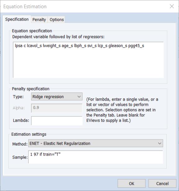
We begin with a simple ridge regression example. Open the equation estimation dialog, select in the drop-down menu, and fill out the dialog as follows:
We list the dependent variable followed by standardized variables as regressors
lpsa c lcavol_s lweight_s age_s lbph_s svi_s lcp_s gleason_s pgg45_s
in the edit field, and choose in the Type drop-down menu.
• We leave the edit field blank so that EViews will determine the lambda path of values to consider.
• We set the estimation sample to the observations where the TRAIN series takes the value “T”.
• On the tab we change the drop-down to since the data are pre-scaled.
• We change the to 0.0001.
We will leave the remaining settings at their defaults. Click on to estimate the equation. EViews will display the main estimation output.
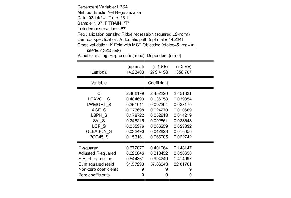
The top portion of the output shows that we are estimating a ridge regression model with automatic path estimation. The optimal value of 14.23403 is computed from 5-fold cross-validation using a mean square error objective. Since the regressors are already standardized, we have specified no regressor scaling and there is no dependent variable scaling.
The output shows the results for estimation using the optimal penalty of 61.62 and the largest penalty values (279.4198 and 1358.707) with cross-validation mean square errors that are 1 and 2 standard deviations from the mean.
In all three cases, all of the coefficients are included in the specification, as expected for ridge regression, and the results clearly show the reduction in both the coefficient values and the goodness of fit measures as we increase the value of

.
Click on to show the coefficients plotted against various values in the graph:
i
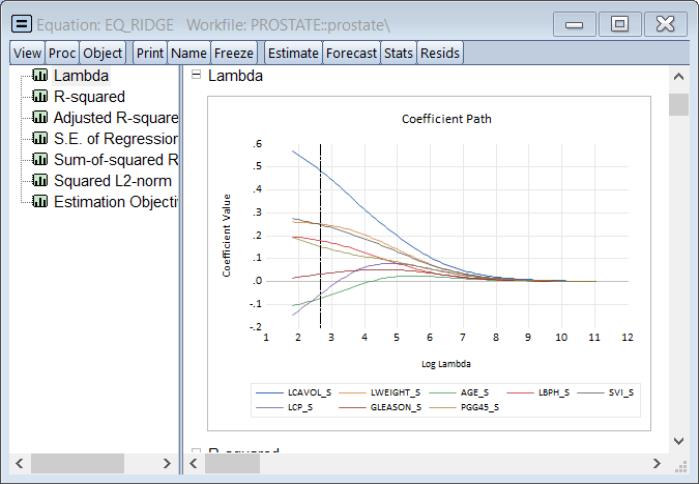
The vertical line shows the optimal value for log

.
We may also see the relationship between the penalty and the fit measures. Select and select the node to see the relationship between the

and the squared deviation based measure of fit:
Note that both measures are monotonically decreasing in the penalty, and the adjusted

is negative for larger values.
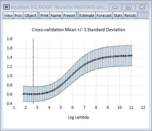
The cross-validation views provide more insight into the effect of increasing penalty. Click on to show the cross-validation objective plotted against the penalty:
The plot shows the average mean square error obtained from the K-fold cross-validation, again with the vertical line corresponding to the optimal log

.
Lasso
Next, we estimate a modified specification using the Lasso penalty function. We change the penalty specification to , and fill out the main estimation dialog with the same variables as before, but increasing the relative penalty of PGG45_S, by entering
lpsa c lcavol_s lweight_s age_s lbph_s svi_s lcp_s gleason_s @vw(pgg45_s, 1.2)
into the edit field.
We use here the simple form of the
@vw specification in which the single argument is assumed to be the weight value. Note that we set individual weight

for PGG45_S to 1.2, so that the variable is more heavily penalized. EViews will apply the specified weight, and then normalize all of the non-zero weights so that they sum to the number of penalized variables.
For added clarity, we may alter the specification to use the option form of the weight specification:
lpsa c lcavol_s lweight_s age_s lbph_s svi_s lcp_s gleason_s @vw(pgg45_s, w=1.2)
All of the remaining settings are as in the original ridge regression example in
“Ridge Regression”.
Click on to estimate the equation.
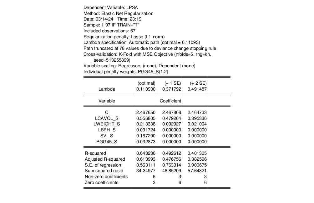
The top of the output is mostly familiar, but has an added line noting the higher individual penalty weight for PGG45_S.
As expected, the Lasso penalty produces more 0-valued coefficients than does the ridge penalty. The main estimation output table drops AGE_S, LCP_S and GLEASON_S from the display since the corresponding coefficient is 0 for all three models. As the penalty increases in the rightward columns, additional coefficients are set to 0. For a

of 0.491487, the only remaining coefficients are for the unpenalized intercept, LCAVOL_S, and LWEIGHT_S.
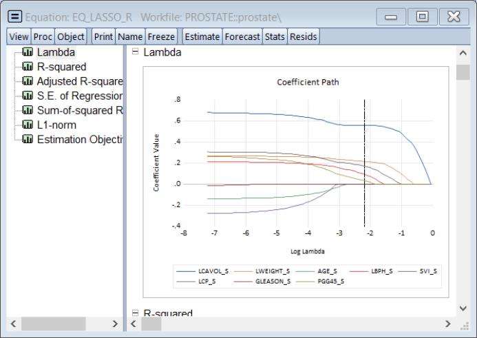
Selecting and examining the graph shows the coefficients plotted against various values of the penalty parameter:
Of particular interest are the values of log lambda where the lines intersect the horizontal axis. We see, for example, that GLEASON_S is the first variable to drop out as we increase the penalty, followed significantly later by LCP_S and then AGE_S. The remaining variables have coefficients which reach zero only at log

values greater than the optimum.
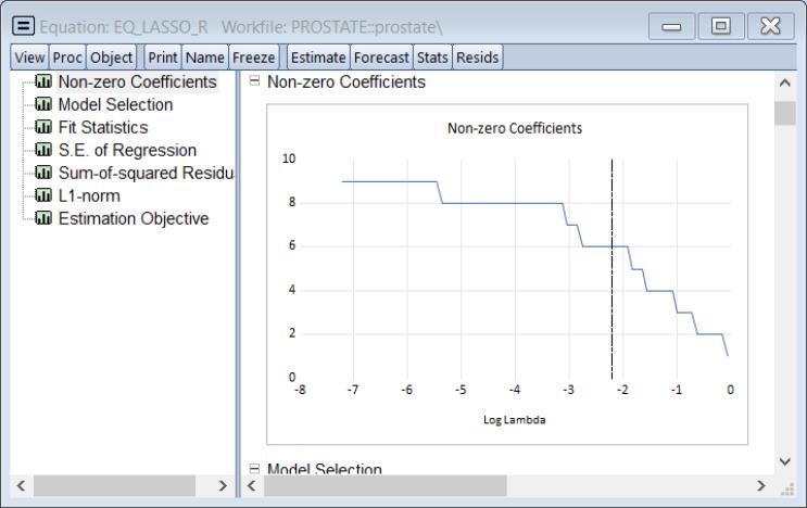
We can see an overview of this behavior by looking at the graph of the number of non-zero coefficients against the values of log

(:
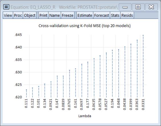
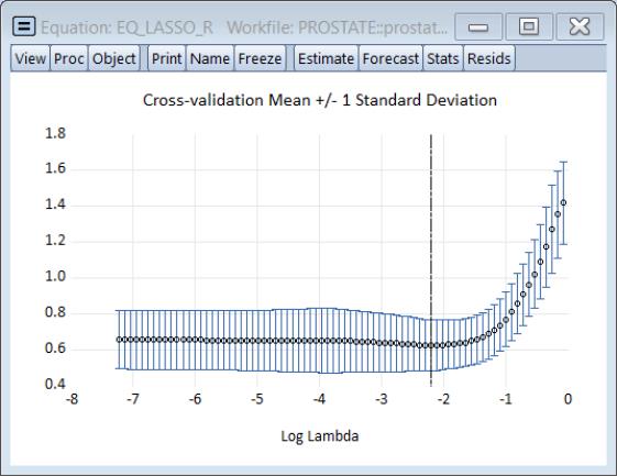
Looking at the cross-validation results shows the behavior of the top 20 models
and shows the behavior of the cross-validation objective along the path.
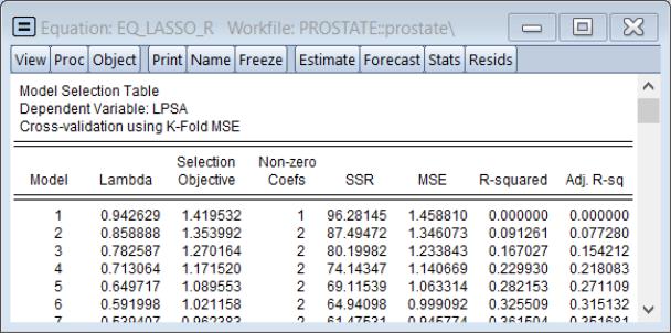
The cross-validation table results () show the objective and various measures of fit for all of the values of the penalty:
Elastic Net
To estimate this model, open the elastic net dialog and fill it out as depicted:
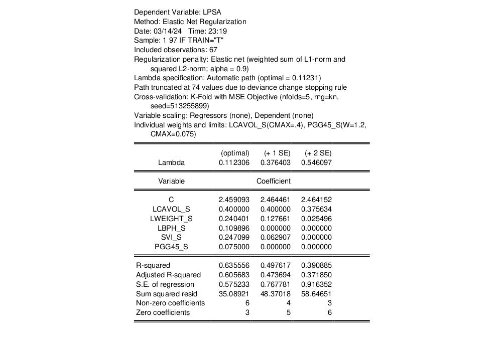
lpsa c lcavol_s lweight_s @vw(age_s, cmax=0.4) lbph_s svi_s lcp_s gleason_s @vw(pgg45_s, cmax=0.1, w=1.2)
In this specification, we restrict the AGE_S variable to have a coefficient less than or equal to 0.4, and we assign an individual weight to PGG45_S of 1.2, with a coefficient maximum value of 0.1.
Again, we leave the edit field blank so that EViews will determine the lambda path of values to consider and we set the estimation sample to the observations where the TRAIN series takes the value “T”. The remaining settings are as in the original ridge regression example in
“Ridge Regression”.
Click on to estimate the equation.
The output should be familiar. Note the line in the header displaying the individual weights and coefficient limits for LCAVOL_S and PGG45_S.
We see here that the upper coefficient limit is binding for LCAVOL_S at both the optimal and the “+1 SE” penalties, but that at the “+2 SE” penalty, the limit is no longer relevant. The PGG45_S coefficient limit is binding at the optimal, but not for the two higher penalties.
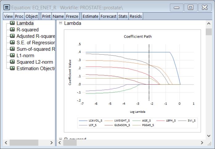
Click on and select the Lambda graph to show the coefficients along the

path:
Notable are the paths of the LCAAVOL_S and the PGG45_S in which the restrictions are binding along the path until the penalty is large enough to shrink the coefficient within the bounds. As expected, as the penalization increases, the complexity of the model decreases and coefficients gradually shrink to 0.
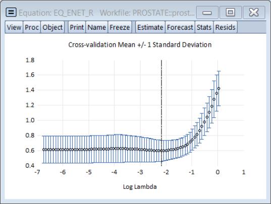
The cross-validation error graph () shows the behavior of the mean square error along the path:

 .
.
 .
. and the squared deviation based measure of fit:
 is negative for larger values.
 .
. for PGG45_S to 1.2, so that the variable is more heavily penalized. EViews will apply the specified weight, and then normalize all of the non-zero weights so that they sum to the number of penalized variables.
 of 0.491487, the only remaining coefficients are for the unpenalized intercept, LCAVOL_S, and LWEIGHT_S.
 values greater than the optimum.
 (View/Lambda Path/Graphs):

 path:
path: 