Post-Estimation Views and Procs
After estimating the model, EViews offers several post-estimation views.
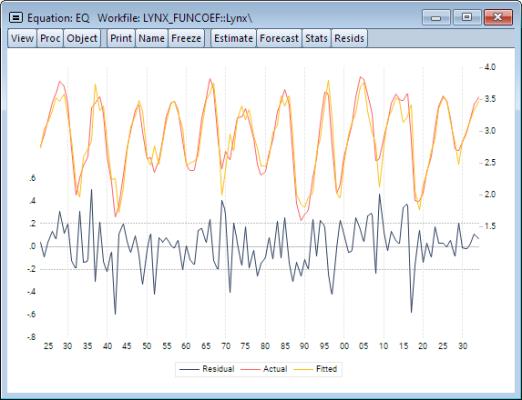
Functional Residuals
You may examine the fitted values and residuals from the fitted model by clicking on and then choosing to display a graph or table view of the residuals, actuals, and fitted values, or a residual graph:
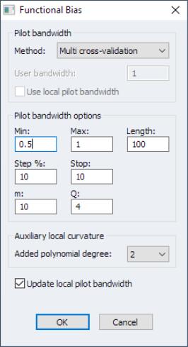
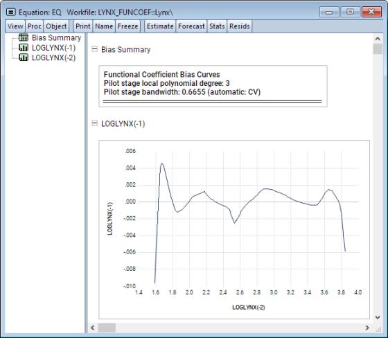
Functional Bias
To display estimates of the functional bias, select from the equation menu. EViews will open a dialog showing you options associated with estimating the bias:
Functional biases must be estimated using a pilot bandwidth (
“Pilot Bandwidth”). The method of selecting a pilot bandwidth for the bias calculation may be specified by selecting desired options. The checkbox may be used to control whether the results of the bandwidth computation are saved as the local pilot.
Alternately, if a pilot bandwidth has previously been set, it may be used for this calculation by clicking on the checkbox (see
“Setting and Clearing the Local Pilot Bandwidth”).
Once your settings have been chosen, click on .
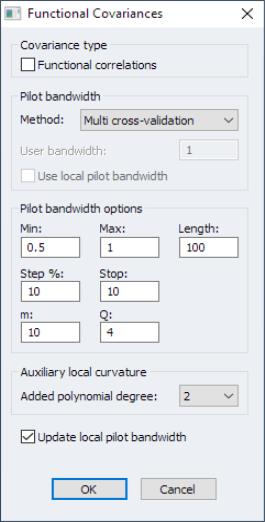
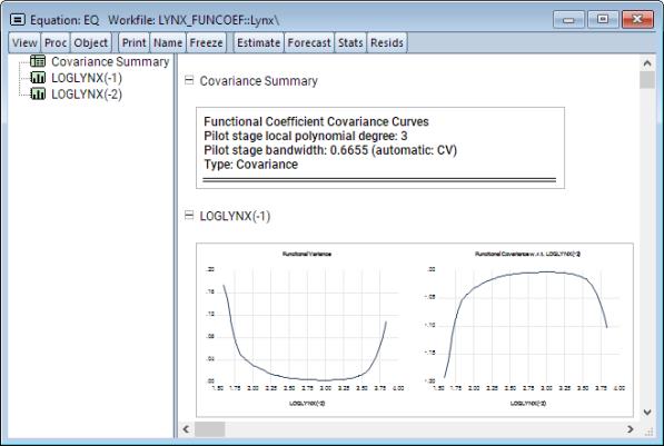
Functional Covariance/Correlation Matrix
Selecting brings up a dialog with options associated with estimating the functional covariance functions:
Functional covariances estimated using a pilot bandwidth (
“Pilot Bandwidth”). A pilot bandwidth for the covariance calculation may be specified using options specified in this dialog. The checkbox may be used to control whether the results of the bandwidth computation are saved as the local pilot.
Alternately, if a pilot bandwidth has previously been set, it may be used for this calculation by clicking on (see
“Setting and Clearing the Local Pilot Bandwidth”).
If you wish to compute correlations instead of covariances, select the checkbox. Click on to display the graphs.
Bandwidth Views
Bandwidth selection is a critical part of functional coefficient estimation. EViews offers views for examining your estimation and pilot bandwidth choices.
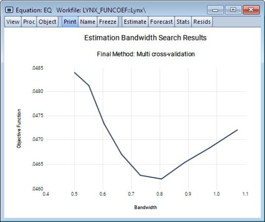
Estimation Bandwidth
To see how the estimation objective function changes along the bandwidth search grid, select or . Selecting the graph, we have:
shows the graph displaying the relationship between the final bandwidth and the value of the objective.
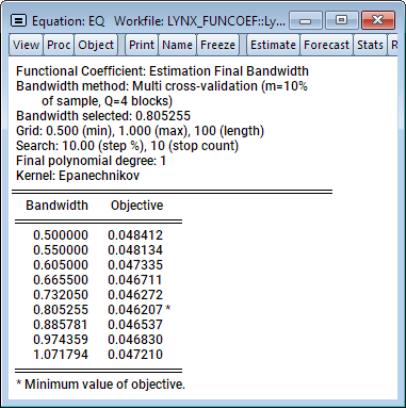
The table display provides an alternative view of the relationship:
If the estimation required computation of a pilot bandwidth, the graph or table will also display the relationship between both the final and the pilot bandwidths and the objective.
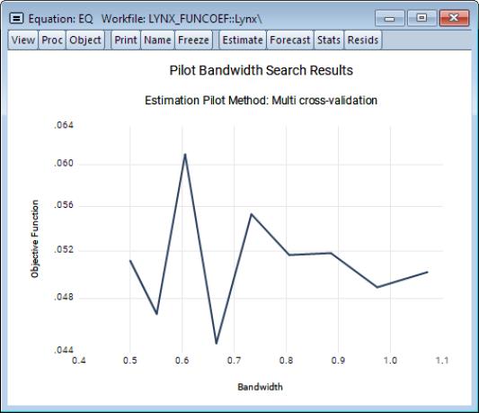
Pilot Bandwidth
To see how the estimation objective function changes along the pilot search grid, select or .
These views will display the pilot bandwidth from estimation, if available, and the local pilot bandwidth, if available (see
“Setting and Clearing the Local Pilot Bandwidth”).
Confidence Intervals
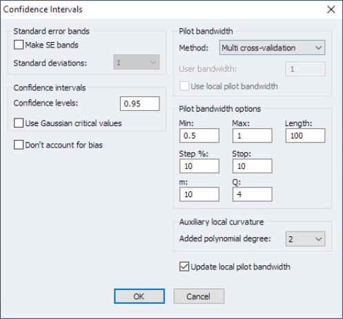
Clicking on brings up a dialog prompting you to specify options for computing the confidence interval and the pilot bandwidth:
The left-hand side of the dialog contains options associated with computation of the confidence intervals.
• If you prefer to compute standard error bands in place of confidence intervals, click on the checkbox and select the number of standard error bands to display in the dropbox.
• If instead you are computing confidence intervals, you may specify one or more levels in the textbox. The default value is 0.95.
• If critical values are to be computed from Gaussian critical values as opposed to the true limiting distribution, check the box.
• Finally, if bias is to be ignored in deriving confidence intervals, select the setting.
The right portion of the dialog shows options associated with the required pilot stage estimation. You may specify pilot bandwidth options in this dialog or choose to use a previously determined local pilot bandwidth (see
“Setting and Clearing the Local Pilot Bandwidth”).
Click on to display the output.
Stability and Significance Tests
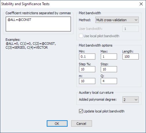
Selecting brings up a dialog prompting you specify the tests and options of interest:
You may provide one or more restrictions specify a test for:
• whether coefficient  is functionally equivalent to a specific numeric value (example, “c(1) = 2”).
 • whether coefficient  is constant on the estimated grid (using the
 keyword; example, “c(1)=@const”).
• whether coefficient  is equal to the values in a series in the workfile (example, “c(1)=s1”).
 • whether coefficient  is equal to the values in a vector in the workfile (for estimation on a custom grid; example “c(1)=v1”).
 • whether all coefficients are restricted (using the keyword; examples, “@all=2”, “@all=@const”).
The remainder of the dialog is reserved for options associated with the pilot stage estimation. You may specify pilot options in this dialog or choose to use a previously determined local pilot bandwidth (see
“Setting and Clearing the Local Pilot Bandwidth”).
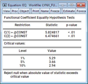
When all options have been specified, click on to display the table of results:
Forecasting
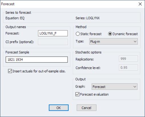
To perform a forecast using the estimated functional coefficient model, click on the button in the equation object, or click on to display the forecast dialog:
Most of these options should be familiar from typical forecast dialogs. The most important difference lies in the choice of forecast . You may use the dropdown to choose between , , , and methods (see
“Point Forecasts” for discussion).
The available computation options depend on the type selected:
• For the Monte Carlo and bootstrap methods, the number of simulations may be set in the textbox.
• When the stochastic method employs a bootstrap, problematic re-sampling of the functional coefficient variable values can be mitigated by selecting the lower and upper data proportions to conform re-sampled observations to said range of original observations.
• For the full bootstrap, computationally complexity can be achieved by choosing to bootstrap only the dependent variable by ensuring the box is checked.
• Finally, when any of the stochastic methods is employed (other than ) is chosen, forecast confidence levels will be derived from the distribution of the simulation results. You may specify the confidence interval level in the edit field. You will also be prompted to enter a name in the edit field to save the confidence intervals in the workfile using names formed by appending “_LWR” and “_UPR” to the specified prefix).
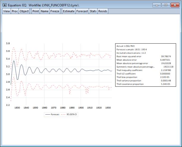
Once all the options are specified, click on to compute the forecasts and display the results.
Setting and Clearing the Local Pilot Bandwidth
Many of the functional coefficient equation views and procedures rely on preliminary computation using a pilot bandwidth. For each of those views and procs, the corresponding dialog offers settings which allow you to specify a method for computing the pilot bandwidth.
A pilot bandwidth may, however, be expensive to compute, and it makes sense to allow users to define a local pilot bandwidth that is computed once and then made available for use in all of subsequent views and procedures.
The local pilot bandwidth may be set in two distinct ways:
• By default, when a estimation final stage bandwidth procedure such as MSE, LOO, or non-parametric AIC is employed, the local pilot bandwidth will be initialized to the pilot bandwidth obtained in that procedure.
(For other estimation methods, no pilot bandwidth is computed so the local pilot bandwidth is not initially defined.)
• You may use the proc to initialize (or replace) the local pilot bandwidth.
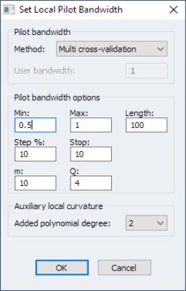
To set the local pilot bandwidth, click on from the equation menu to display the dialog:
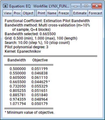
From here, select the desired options and click on to compute and save a local pilot bandwidth and to display a summary of the bandwidth selection results:
The local pilot bandwidth will be available in all views and procs that employ a pilot bandwidth. You may elect to use this bandwidth in those cases by selecting the checkbox.
You may display a table or a graph of both the estimation pilot bandwidth (if available) and the local pilot bandwidth results by clicking on and selecting either or (
“Bandwidth Views”).
To clear the local pilot bandwidth, select
Output Objects to Workfile
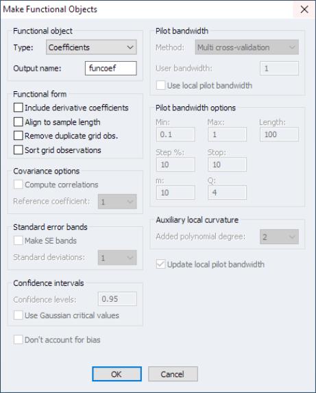
Selecting allows you to export various functional coefficients results to the workfile:
The type of functional object to be saved may be chosen from the dropdown. In most cases, you will be prompted for an to be used in saving the object to the workfile.
The output of the functional object is saved to a matrix in the workfile where the rows correspond to the evaluation points specified in estimation. If estimation uses the default evaluation grid, functional values will be computed at the data values of the functional coefficient series for each observation in the estimation sample. Alternately, if you specified a uniform grid or provided a workfile vector, the rows will correspond to the elements of that custom grid.
There are several options associated with the composition of this matrix:
• You should check box if you the wish to expand the number of rows of the output matrix are to match the workfile length. Aligning the rows of the output matrix to match the workfile will make it easier to export the results to series.
• Duplicate evaluation points are sometimes present in series or vector-based functional coefficient evaluation. If you wish to only evaluate the functional values at unique points, you should click on the checkbox.
• By default, the rows of the matrix will contain evaluation point values as they are observed. For series or vector-based functional coefficient evaluation, the rows will therefore be unordered with respect to these values. If you wish to sort the rows by the evaluation point values, select the checkbox. The rows of the output matrix will be ordered from low to high values of the evaluation points.
Recall that the Taylor expansion in
Equation (38.5) creates coefficients associated with the degree of the expansion. By default EViews will save only the original equation coefficients, but you may elect to save results associated these derivatives:
• To include derivative coefficient results in the output, check the box.
For each output type, there will be different available options:
• When the output object requires a pilot bandwidth for computation, the will be displayed.
• Covariances and correlations are produced with respect to some reference coefficient which should be specified in the dropdown.
• For confidence intervals, the options associated with computation of confidence intervals or standard errors will be displayed (
“Confidence Intervals”). Note that the confidence intervals for coefficients will be saved in pairs to adjacent columns of the output matrix.
The remaining portion of the dialog shows options associated with the required pilot stage estimation. You may specify pilot bandwidth options in this dialog or choose to use a previously determined local pilot bandwidth (see
“Setting and Clearing the Local Pilot Bandwidth”).