How to Estimate a GLM in EViews
To estimate a GLM model in EViews you must first create an equation object. You may select or from the main menu, or enter the keyword equation in the command window. Next select in the dropdown menu. Alternately, entering the keyword glm in the command window will both create the object and automatically set the estimation method. The dialog will change to show settings appropriate for specifying a GLM.
Specification
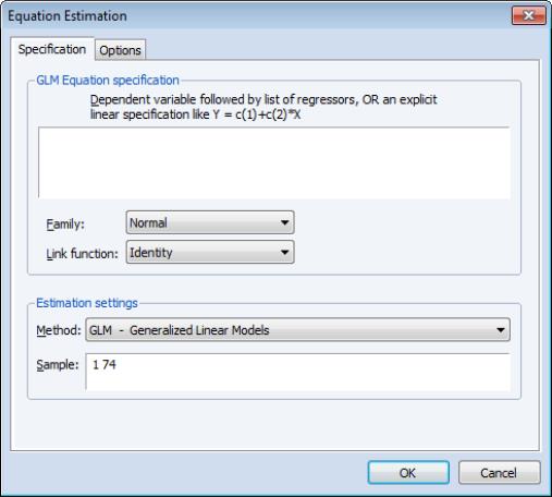
The main page of the dialog is used to describe the basic GLM specification.
We will focus attention on the section since the section in the bottom of the dialog is should be self-explanatory.
Dependent Variable and Linear Predictor
In the main edit field you should specify your dependent variable and the linear predictor.
There are two ways in which you may enter this information. The easiest method is to list the dependent response variable followed by all of the regressors that enter into the predictor. PDL specifications are permitted in this list, but ARMA terms are not. If you wish to include an offset in your predictor, it should be entered on the page (see
“Specification Options”).
Alternately, you may enter an explicit linear specification like “Y=C(1)+C(2)*X”. The response variable will be taken to be the variable on the left-hand side of the equality (“Y”) and the linear predictor will be taken from the right-hand side of the expression (“C(1)+C(2)*X”). Offsets may be entered directly in the expression or they may be entered on the page. Note that this specification should not be taken as a literal description of the mean equation; it is merely a convenient syntax for specifying both the response and the linear predictor.
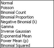
Family
Next, you should use the dropdown to specify your distribution. The default family is the distribution, but you are free to choose from the list of linear exponential family and quasi-likelihood distributions. Note that the last three entries (, , ) are for quasi-likelihood specifications not associated with exponential families.
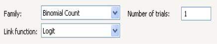
If the selected distribution requires specification of an ancillary parameter, you will be prompted to provide the values. For example, the and distributions both require specification of the number of trials

, while the requires specification of the excess-variance parameter

.
For descriptions of the various exponential and quasi-likelihood families, see
“Distribution”.
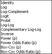
Link
Lastly, you should use the dropdown to specify a link function.
EViews will initialize the setting to the default for to the selected family. In general, the canonical link is used as the default link, however, the link is used as the default for the family. The , , and quasi-likelihood families will default to use the , , and links, respectively.
If the link that you select requires specification of parameter values, you will be prompted to enter the values.
For detailed descriptions of the link functions, see
“Link”.
Options
Click on the tab to display additional settings for the GLM specification. You may use this page to augment the equation specification, to choose a dispersion estimator, to specify the estimation algorithm and associated settings, or to define a coefficient covariance estimator.
Specification Options
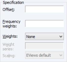
The section of the tab allows you to augment the GLM specification.
To include an offset in your linear predictor, simply enter a series name or expression in the edit field.
The edit field should be used to specify replicates for each observation in the workfile. In practical terms, the frequency weights act as a form of variance weighting and inflate the number of “observations” associated with the data records.
You may also specify prior variance weights in the using the dropdown and associated edit fields. To specify your weights, simply select a description for the form of the weighting series (, , , ), then enter the corresponding weight series name or expression. EViews will translate the values in the weighting series into the appropriate values for

. For example, to specify

directly, you should select then enter the series or expression containing the

values. If you instead choose , EViews will set

to the inverse of the values in the weight series.
“Weighted Least Squares” for additional discussion.
Dispersion Options
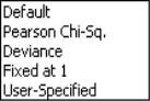
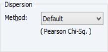
The dropdown may be used to select the dispersion computation method. You will always be given the opportunity to choose between the setting or , , and . Additionally, if the specified distribution is in the linear exponential family, you may choose to use the statistic.
The entry instructs EViews to use the default method for computing the dispersion, which will depend on the specified family. For families with a free dispersion parameter, the default is to use the statistic, otherwise the default is . The current default setting will be displayed directly below the dropdown.
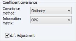
Coefficient Covariance Options
The dropdown specifies the estimator for the coefficient covariance matrix. You may choose between the method, which uses the inverse of the estimated information matrix, or you may elect to use sandwich estimator, the heteroskedasticity and auto-correlation consistent approach, or a Cluster-robust QML sandwich estimator.
If you select the HAC covariance method, a HAC options button will appear prompting so that you may customize the whitening and kernel settings. By default, EViews HAC estimation will employ a Bartlett kernel with fixed Newey-West sample-size based bandwidth and no pre-whitening (see
“HAC Consistent Covariances (Newey-West)” for additional discussion).
If you select the cluster-robust method, an edit field will prompt you for the cluster identifier variable.
The dropdown allows you to specify the method for estimating the information matrix. For covariances computed in the standard fashion, you may choose between the default , , and . If you are computing Huber/White covariances, only the two Hessian based selections will be displayed.
(Note that in some earlier versions of EViews, the information matrix default method was tied in with the optimization method. This default dependence has been eliminated.)
Lastly you may use the checkbox choose whether to apply a degree-of-freedom correction to the coefficient covariance. By default, EViews will perform this adjustment.
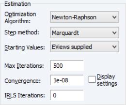
Estimation Options
The section of the page lets you specify the optimization algorithm, starting values, and other estimation settings.
The and dropdown menus control your estimation method.
• The default is , but you may instead select , , (IRLS), or .
• The default is , but you may use the menu to select or .
If you select optimization using , you will be prompted to select a legacy method in place of a step method. The dropdown offers the choice of the default (Newton-Raphson with Marquardt steps), with line search, , and (OPG with line search).
By default, the dropdown is set to . The EViews default starting values for

are obtained using the suggestion of McCullagh and Nelder to initialize the IRLS algorithm at
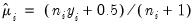
for the binomial proportion family, and
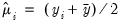
otherwise, then running a single IRLS coefficient update to obtain the initial

. Alternately, you may specify starting values that are a fraction of the default values, or you may instruct EViews to use your own values.
You may use the edit field to instruct EViews to perform a fixed number of additional IRLS updates to refine coefficient values prior to starting the specified estimation algorithm.
The and edit fields are self-explanatory. Selecting the checkbox instructs EViews to show detailed information on tolerances and initial values in the equation output.
Coefficient Name
You may use the Coefficient name section of the dialog to change the coefficient vector from the default C. EViews will create and resize the vector if necessary.