Covariance Analysis
The covariance analysis view may be used to obtain different measures of association (covariances and correlations) and associated test statistics for the series in a group. You may compute measures of association from the following general classes:
• ordinary (Pearson product moment)
• ordinary uncentered
• Spearman rank-order
• Kendall’s tau-a and tau-b
EViews allows you to calculate partial covariances and correlations for each of these general classes, to compute using balanced or pairwise designs, and to weight individual observations. In addition, you may display your results in a variety of formats and save results to the workfile for further analysis.
Performing Covariance Analysis
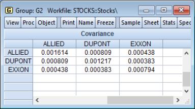
We consider the stock price example from Johnson and Wichern (1992, p. 397) in which 100 observations on weekly rates of return for Allied Chemical, DuPont, Union Carbide, Exxon, and Texaco were examined over the period from January 1975 to December 1976 (“Stocks.WF1”). These data are in the group object G2 containing the series ALLIED, DUPONT, UNION.
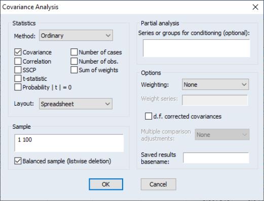
To proceed, simply open the group object and select to display the covariance dialog:
We will consider the various options in detail below. For now, note that by default, EViews will compute the unweighted ordinary (Pearson product moment) covariance for the data in the group, and display the result in a spreadsheet view.
The current sample of observations in the workfile, “1 100”, will be used by default, and EViews will perform listwise exclusion of cases with missing values to balance the sample if necessary.
Click on to accept the defaults, and the group display changes to show the covariances between the variables in the group. The sheet header clearly shows that we have computed the covariances for the data. Each cell of the table shows the variances and covariances for the corresponding variables. We see that the rates of return are positively related, though it is difficult to tell at a glance the relative strengths of the relationships.
Statistics
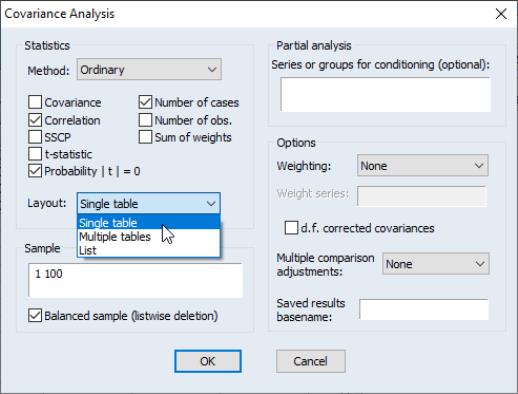
Let us now consider some of the options in the dialog in greater detail. The first section of the dialog, labeled , controls the statistics to be calculated, and the method of displaying our results.
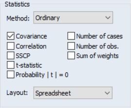
First you may use the dropdown to specify the type of calculations you wish to perform. You may choose between computing ordinary Pearson covariances (), uncentered covariances (), Spearman rank-order covariances (), and Kendall’s tau measures of association ().
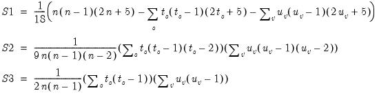
The checkboxes below the dropdown menu identify the statistics to be computed. Most of the statistics are self-explanatory, but a few deserve a quick mention
The statistic labeled refers to the “sum-of-squared cross-products.” The is the number of rows of data used in computing the statistics, while the N is the obviously the number of observations employed. These two values will differ only if frequency weights are employed. The will differ from the number of cases only if weighting is employed, and it will differ from the number of observations only if weights are non-frequency weights.
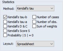
If you select from the dropdown, the checkbox area changes to provide you with choices for a different set of covariance statistics. In addition to the previously offered number of cases and obs, and the sum of weights, EViews allows you to display Kendall’s tau-a and tau-b, the raw concordances and discordances, Kendall’s score statistic, and the probability value for the score statistic.
Turning to the layout options, EViews provides you with up to four display options: , , , and . We have already seen the spreadsheet view of the statistics. As the names suggest, the two table views lay out the statistics in a table view; the single table will stack multiple statistics in a single “cell” of the table, while the multiple tables will place the table for the second statistic under the table for the first statistic, etc. The list view displays each of the statistics in a separate column of a table, with the rows corresponding to pairs of variables. Note that the spreadsheet view is not available if you select multiple statistics for display.
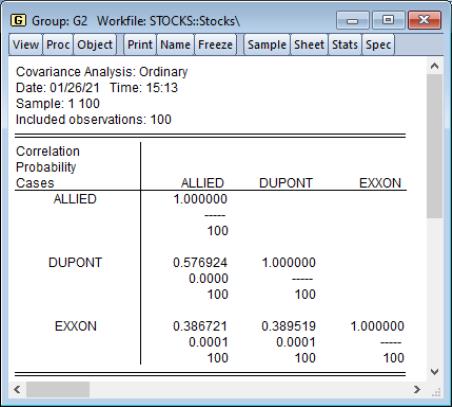
In this example, we perform ordinary covariance analysis and display multiple statistics in a single table. We see that all of the correlations are positive, and significantly different from zero at conventional levels. Displaying the instead of makes it easier to see that the two chemical companies, Allied and DuPont are more highly correlated with each other than they are with the oil company Exxon.
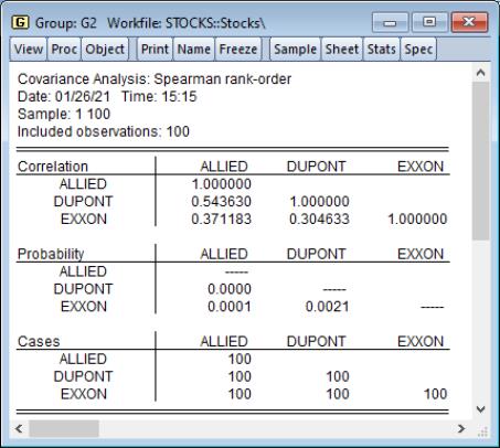
To compute Spearman rank-order correlations, simply select in the dropdown and choose the statistics you wish to compute. Spearman rank-order covariances is a nonparametric measure of correlation that may be thought of as ordinary covariances applied to rank transformed data. Here we display three Spearman results, , , and , arranged in :
Note that the multiple table results make it easier to compare correlations across variables, but more difficult to relate a given correlation to the corresponding probability and number of cases.
A third major class of measures of association is based on Kendall’s tau (see
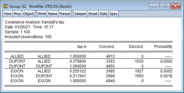
“Kendall’s Tau”). Briefly, Kendall’s tau for two variables is based on the number of concordances and discordances between the orderings of the variables for all possible comparisons of observations. If the number of concordances and discordances are roughly the same, there is no association between the variables, relatively large numbers of concordances suggest a positive relationship between the variables, and conversely for relatively large numbers of discordances.
Here, we display output in list format, showing , , and :
The results are similar to those obtained from ordinary and Spearman correlations, though the tau-b measures of association are somewhat lower than their counterparts.
Sample
EViews will initialize the edit field with the current workfile sample, but you may modify the entry as desired.
By default, EViews will perform listwise deletion when it encounters missing values so that all statistics are calculated using the same observations. To perform pairwise deletion of missing values, simply uncheck the checkbox. Pairwise calculations will use the maximum number of observations for each calculation.
Note that this option will be ignored when performing partial analysis since the latter is only performed on balanced samples
Partial Analysis
A partial covariance is the covariance between two variables while controlling for a set of conditioning variables.
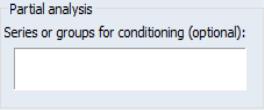
To perform partial covariance analysis in EViews, simply enter a list of conditioning variables in the partial analysis edit field. EViews will automatically balance the sample, compute the statistics and display the results. Partial covariances or correlations will be computed for each pair of analysis variables, controlling for all of the variables in the conditioning set.
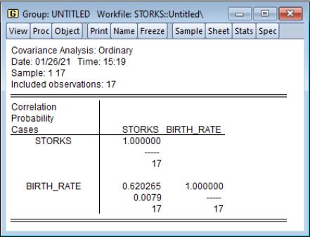
Consider the example from Matthews (2000) in which we consider the Pearson correlation between the number of stork breeding pairs and the number of births in 17 European countries. The data are provided in the workfile “Storks.WF1”.
The unconditional correlation coefficient of 0.62 for the STORKS and BIRTH_RATE variables is statistically significant, with a p-value of about 0.008, indicating that the numbers of storks and the numbers of babies are correlated.
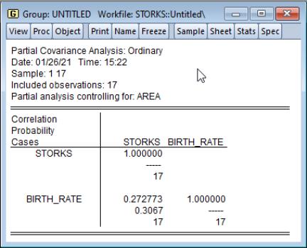
While some stork lovers may wish to view this correlation as indicative of a real relationship, others might argue that the positive correlation is spurious. One possible explanation lies in the existence of confounding variables or factors which are related to both the stork population and the number of births. Two possible factors are the population and area of the country.
To perform the analysis conditioning on the country area, select the statistics you wish to display, enter AREA in the partial analysis edit field, and press . The partial correlation falls to 0.27, with a statistically insignificant p-value of about 0.31.
Options
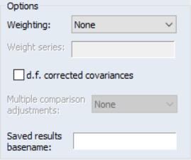
EViews provides a variety of other options for calculating your measures of association and for saving results.
Weighting
When you specify weighting, you will be prompted to enter a different weighting method and the name of a weight series. There are five different weight choices: frequency, variance, standard deviation, scaled variance, and scaled standard deviation.
EViews will compute weighted means and variances using the specified series and weight method. In each case, observations are weighted using the weight series; the different weight choices correspond to different functions of the series and different numbers of observations.
See
“Weighting” for details.
Degrees-of-freedom Correction
You may choose to compute covariances using the maximum likelihood estimator or using the unbiased (degree-of-freedom corrected) formula. By default, EViews computes the ML estimates of the covariances.
When you check , EViews will compute the covariances by dividing the sums-of-squared cross-products by the number of observations

less the number of conditioning elements

, where

equals the number of conditioning variables, including the mean adjustment term, if present. For example, if you compute ordinary covariances conditional on

, the divisor will be

.
Multiple Comparison Adjustments
You may adjust your probability values for planned multiple comparisons using Bonferroni or Dunn-Sidak adjustments. In both of these approaches you employ a conservative approach to testing by adjusting the level of significance for each comparison so that the overall error does not exceed the nominal size.
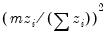
The Bonferroni adjustment sets the elementwise size to
 | (12.1) |
where

is the specified (overall) size of the tests, and

is the number of tests performed. For the Dunn-Sidak adjustment, we set the elementwise size to
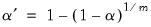 | (12.2) |
For details, see Sokal and Rohlf (1995, p. 228–240).
Saved Results
You may place the results of the covariance analysis into symmetric matrices in the workfile by specifying a . For each requested statistic, EViews will save the results in a sym matrix named by appending an identifier (“cov,” “corr,” “sscp,” “tstat,” “prob,” “taua,” “taub,” “score” (Kendall’s score), “conc” (Kendall’s concurrences), “disc” (Kendall’s discordances), “cases,” “obs,” “wgts”) to the basename.
For example, if you request ordinary correlations, probability values, and number of observations, and enter “MY” in the edit field, EViews will output three sym matrices MYCORR, MYPROB, MYOBS containing the results. If objects with the specified names already exist, you will be prompted to replace them.
Details
The following is a brief discussion of computational details. For additional discussion, see Johnson and Wichern (1992), Sheskin (1997), Conover (1980), and Kendall and Gibbons (1990).
Ordinary and Uncentered Covariances
The sums-of-squared cross-products are computed using
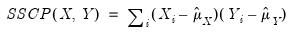 | (12.3) |
where

and

are the estimates of the means. For uncentered calculations, the mean estimates will be set to 0.
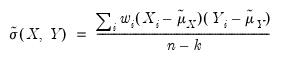
The covariances are computed by dividing the SSCP by the number of observations with or without a degrees-of-freedom correction:
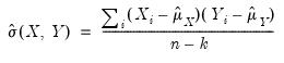 | (12.4) |
where

is the number of observations associated with the observed

,

pairs, and

is a degree-of-freedom adjustment term. By default EViews uses the ML estimator so that

, but you may perform a degrees-of-freedom correction that sets

equal to the number of conditioning variables (including of the mean adjustment term, if present).
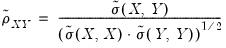
The correlation between the variables

and

is computed from the following expression:
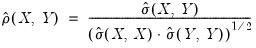 | (12.5) |
It is worth reminding you that in unbalanced designs, the numbers of observations used in estimating each of the moments may not be the same.
Spearman Rank-order Covariances
Spearman covariances are a nonparametric measure of association that is obtained by computing ordinary covariances on ranked data, where ties are handled using averaging. To compute the Spearman rank-order covariances and correlations, we simply convert the data to ranks and then compute the centered ordinary counterparts.
Textbooks often provide simplified expressions for the rank correlation in to the case where there are no ties. In this case,
Equation (12.5) simplifies to:
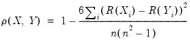 | (12.6) |
where

returns the rank of the observation.
Kendall’s Tau
Kendall’s tau is a nonparametric statistic that, like Spearman’s rank-order statistic, is based on the ranked data. Unlike Spearman’s statistic, Kendall’s tau uses only the relative orderings of ranks and not the numeric values of the ranks.
Consider the ranked data for any two observations

and

. We say that there is a
concordance in the rankings if the relative orderings of the ranks for the two variables across observations are the same:

and

or
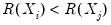
and
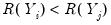
. Conversely, we say that there is a
discordance if the ordering of the

ranks differs from the ordering of the

ranks:
and

or

and
. If there are ties in the ranks of either the

or the

pairs, we say the observation is neither concordant or discordant.
Intuitively, if

and

are positively correlated, the number of concordances should outnumber the number of discordances. The converse should hold if

and

are negatively related.
We may form a simple measure of the relationship between the variables by considering Kendall’s score

, defined as the excess of the concordant pairs,

, over the discordant pairs,

.

which may be expressed as:
 | (12.7) |
where the sign function takes the values -1, 0, and 1 depending on whether its argument is negative, zero, or positive. Kendall’s tau-a is defined as the average of the excess of the concordant over the discordant pairs. There are

unique comparisons of pairs of observations that are possible so that:
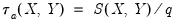 | (12.8) |
In the absence of tied ranks,

, with

when all pairs are concordant and

when all pairs are discordant.
One disadvantage of

is that the endpoint values -1 and 1 are not reached in the presence of tied ranks. Kendall’s tau-b

rescales

by adjusting the denominator of

to account for the ties:
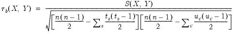 | (12.9) |
where

are the number of observations tied at each unique rank of

, and

are the number of observations tied at each rank of

. This rescaling ensures that
. Note that in the absence of ties, the summation terms involving

and

equal zero so that

.
It is worth noting that computation of these measures requires

comparisons, a number which increases rapidly with

. As a result, textbooks sometimes warn users about computing Kendall’s tau for moderate to large samples. EViews uses very efficient algorithms for this computation, so for practical purposes, the warning may safely be ignored. If you find that the computation is taking too long, pressing the ESC break key may be used to stop the computation.
Weighting
Suppose that our weight series

has

individual
cases denoted by

. Then the weights and number of observations associated with each of the possible weighting methods are given by:
| | |
Frequency | | |
Variance | | |
Std. Dev. | | |
Scaled Variance | | |
Scaled Std. Dev. | | |
Frequency weighting is the only weighting allowed for Spearman’s rank-order and Kendall’s tau measures of association.
The weighted SSCP is given by
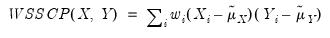 | (12.10) |
where the

and

are the original data or ranks (respectively), the

are weighted means (or zeros if computing uncentered covariances), and the

are weights that are functions of the specified weight series.
If estimated, the weighted means of

and

are given by:
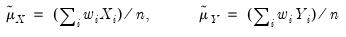 | (12.11) |
where

is the number of observations.
The weighted variances are given by
 | (12.12) |
and the weighted correlations by
 | (12.13) |
The weighted Kendall’s tau measures are derived by implicitly expanding the data to accommodate the repeated observations, and then evaluating the number of concordances and discordances in the usual fashion.
Testing
The test statistics and associated
p-values reported by EViews are for testing the hypothesis that a single correlation coefficient is equal to zero. If specified, the
p-values will be adjusted using Bonferroni or Dunn-Sidak methods (see
“Multiple Comparison Adjustments”).
For ordinary Pearson and Spearman correlations, the t-statistic is computed as
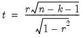 | (12.14) |
where

is the estimated correlation, and

is the number of conditioning variables, including the implicit mean adjustment term, if necessary. The
p-value is obtained from a
t-distribution with

degrees-of-freedom (Sheskin, 1997, p. 545, 598).
In the leading case of centered non-partial correlations,

, so the degrees-of-freedom is

. For centered partial correlations,

where

is the number of non-redundant conditioning variables, so the degrees of freedom is given by

.
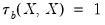
The test of significance for Kendall’s tau is based on a normal approximation using the continuity corrected

-statistic (Kendall and Gibbons, 1990, p. 65–66):
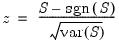 | (12.15) |
where the variance is given by:
 | (12.16) |
for
 | (12.17) |
where

are the number of observations tied at each unique rank of

and

are the number of observations tied at each rank of

. In the absence of ties,
Equation (12.16) reduces to the expression:
 | (12.18) |
usually provided in textbooks (e.g., Sheskin, 1997, p. 633).
Probability values are approximated by evaluating the two-tailed probability of

using the standard normal distribution. Note that this approximation may not be appropriate for small sample sizes; Kendall and Gibbons (1990) suggest that the approximation is not generally recommended for

(in the untied case).
Significance level values are currently not provided for partial Kendall’s tau.
Partial Analysis
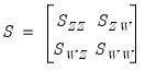
Let

be the set of analysis variables, and let

be the set of conditioning variables.
For the ordinary and Spearman rank-order calculations, the joint sums of squares and cross-products for the two sets of variables are given by:
 | (12.19) |
EViews conditions on the

variables by calculating the partial SSCP using the partitioned inverse formula:
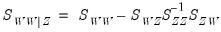 | (12.20) |
In the case where

is not numerically positive definite,

is replaced by a subset of

formed by sequentially adding variables that are not linear combinations of those already included in the subset.
Partial covariances are derived by dividing the partial SSCP by

; partial correlations are derived by applying the usual correlation formula (scaling the partial covariance to unit diagonals).
For Kendall’s tau computations, the partitioned inverse is applied to the corresponding matrix of joint Kendall’s tau values. The partial Kendall’s tau values are obtained by applying the correlation formula to the partitioned inverse.