Binary Dependent Variable Models
In this class of models, the dependent variable,

may take on only two values—

might be a dummy variable representing the occurrence of an event, or a choice between two alternatives. For example, you may be interested in modeling the employment status of each individual in your sample (whether employed or not). The individuals differ in age, educational attainment, race, marital status, and other observable characteristics, which we denote as

. The goal is to quantify the relationship between the individual characteristics and the probability of being employed.
Background
Suppose that a binary dependent variable,

, takes on values of zero and one. A simple linear regression of

on

is not appropriate, since among other things, the implied model of the conditional mean places inappropriate restrictions on the residuals of the model. Furthermore, the fitted value of

from a simple linear regression is not restricted to lie between zero and one.
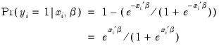
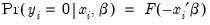
Instead, we adopt a specification that is designed to handle the specific requirements of binary dependent variables. Suppose that we model the probability of observing a value of one as:
 | (31.1) |
where

is a continuous, strictly increasing function that takes a real value and returns a value ranging from zero to one. In this, and the remaining discussion in this chapter follows we adopt the standard simplifying convention of assuming that the index specification is linear in the parameters so that it takes the form

. Note, however, that EViews allows you to estimate models with nonlinear index specifications.
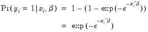
The choice of the function

determines the type of binary model. It follows that:
 | (31.2) |
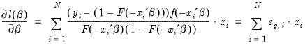
Given such a specification, we can estimate the parameters of this model using the method of maximum likelihood. The likelihood function is given by:
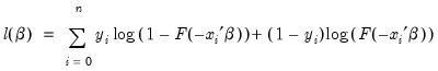 | (31.3) |
The first order conditions for this likelihood are nonlinear so that obtaining parameter estimates requires an iterative solution. By default, EViews uses a second derivative method for iteration and computation of the covariance matrix of the parameter estimates. As discussed below, EViews allows you to override these defaults using the Options dialog (see
“Second Derivative Methods” for additional details on the estimation methods).
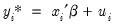
There are two alternative interpretations of this specification that are of interest. First, the binary model is often motivated as a latent variables specification. Suppose that there is an unobserved latent variable

that is linearly related to

:
 | (31.4) |
where

is a random disturbance. Then the observed dependent variable is determined by whether

exceeds a threshold value:
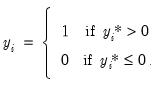 | (31.5) |
In this case, the threshold is set to zero, but the choice of a threshold value is irrelevant, so long as a constant term is included in

. Then:
 | (31.6) |
where

is the cumulative distribution function of

. Common models include probit (standard normal), logit (logistic), and gompit (extreme value) specifications for the

function.
In principle, the coding of the two numerical values of

is not critical since each of the binary responses only represents an event. Nevertheless, EViews requires that you code

as a zero-one variable. This restriction yields a number of advantages. For one, coding the variable in this fashion implies that expected value of

is simply the probability that

:
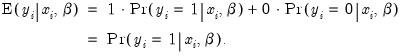 | (31.7) |
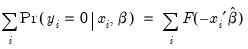
This convention provides us with a second interpretation of the binary specification: as a conditional mean specification. It follows that we can write the binary model as a regression model:
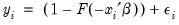 | (31.8) |
where

is a residual representing the deviation of the binary

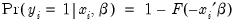
from its conditional mean. Then:
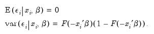 | (31.9) |
We will use the conditional mean interpretation in our discussion of binary model residuals (see
“Make Residual Series”).
Estimating Binary Models in EViews
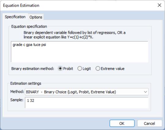
To estimate a binary dependent variable model, choose from the main menu and select the Equation object from the main menu. From the dialog, select the BINARY - Binary Choice (Logit, Probit, Extreme Value) estimation method. The dialog will change to reflect your choice. Alternately, enter the keyword binary in the command line and press ENTER.
There are two parts to the binary model specification. First, in the Equation Specification field, you may type the name of the binary dependent variable followed by a list of regressors or you may enter an explicit expression for the index. Next, select from among the three distributions for your error term:
Probit | where  is the cumulative distribution function of the standard normal distribution. |
Logit | which is based upon the cumulative distribution function for the logistic distribution. |
Extreme value (Gompit) | which is based upon the CDF for the Type-I extreme value distribution. Note that this distribution is skewed. |
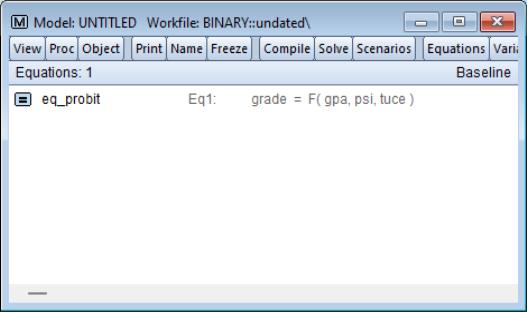
For example, consider the probit specification example described in Greene (2008, p. 781-783) where we analyze the effectiveness of teaching methods on grades. The variable GRADE represents improvement on grades following exposure to the new teaching method PSI (the data are provided in the workfile “Binary.WF1”). Also controlling for alternative measures of knowledge (GPA and TUCE), we have the specification:
Once you have specified the model, click . EViews estimates the parameters of the model using iterative procedures, and will display information in the status line. EViews requires that the dependent variable be coded with the values zero-one with all other observations dropped from the estimation.
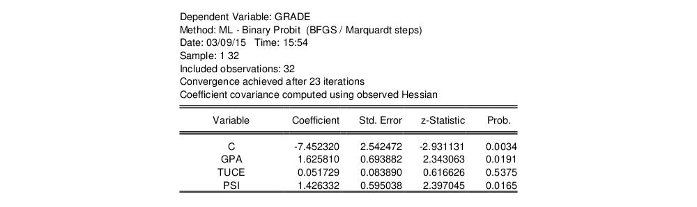
Following estimation, EViews displays results in the equation window. The top part of the estimation output is given by:
The header contains basic information regarding the estimation technique (ML for maximum likelihood) and the sample used in estimation, as well as information on the number of iterations required for convergence, and on the method used to compute the coefficient covariance matrix.
Displayed next are the coefficient estimates, asymptotic standard errors, z-statistics and corresponding p-values.
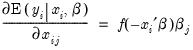
Interpretation of the coefficient values is complicated by the fact that estimated coefficients from a binary model cannot be interpreted as the marginal effect on the dependent variable. The marginal effect of

on the conditional probability is given by:
 | (31.10) |
where
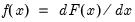
is the density function corresponding to

. Note that

is weighted by a factor

that depends on the values of
all of the regressors in

. The
direction of the effect of a change in

depends only on the sign of the

coefficient. Positive values of

imply that increasing

will increase the probability of the response; negative values imply the opposite.
While marginal effects calculation is not provided as a built-in view or procedure, in
“Forecast”, we show you how to use EViews to compute the marginal effects.
An alternative interpretation of the coefficients results from noting that the ratios of coefficients provide a measure of the relative changes in the probabilities:
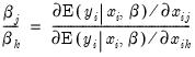 | (31.11) |
In addition to the summary statistics of the dependent variable, EViews also presents the following summary statistics:
First, there are several familiar summary descriptive statistics: the mean and standard deviation of the dependent variable, standard error of the regression, and the sum of the squared residuals. The latter two measures are computed in the usual fashion using the ordinary residuals:
 | (31.12) |
Additionally, there are several likelihood based statistics:
• Log likelihood is the maximized value of the log likelihood function

.
• Avg. log likelihood is the log likelihood

divided by the number of observations

.
• Restr. log likelihood is the maximized log likelihood value, when all slope coefficients are restricted to zero,

. Since the constant term is included, this specification is equivalent to estimating the unconditional mean probability of “success”.
• The
LR statistic tests the joint null hypothesis that all slope coefficients except the constant are zero and is computed as
. This statistic, which is only reported when you include a constant in your specification, is used to test the overall significance of the model. The degrees of freedom is one less than the number of coefficients in the equation, which is the number of restrictions under test.
• Probability(LR stat) is the
p-value of the LR test statistic. Under the null hypothesis, the LR test statistic is asymptotically distributed as a

variable, with degrees of freedom equal to the number of restrictions under test.
• McFadden R-squared is the likelihood ratio index computed as
, where

is the restricted log likelihood. As the name suggests, this is an analog to the

reported in linear regression models. It has the property that it always lies between zero and one.
Estimation Options
The iteration limit, convergence criterion, and coefficient name may be set in the usual fashion by clicking on the tab in the dialog. In addition, there are options that are specific to binary models. These options are described below.
Optimization
By default, EViews uses Newton-Raphson with Marquardt steps to obtain parameter estimates.
If you wish, you can use the dropdown menu to select a different method. In addition to , you may select , , or .
For non-legacy estimation, the may be chosen between Marquardt, Dogleg, and Line search. For legacy estimation the is set to the default (Marquardt steps) or (line search).
Note that for legacy estimation, the default optimization algorithm does influence the default method of computing coefficient covariances.
Coefficient Covariances
For binary dependent variable models, EViews allows you to estimate the standard errors using the default (inverse of the estimated information matrix), quasi-maximum likelihood (Huber/White), cluster quasi-ML (), or generalized linear model (GLM) methods. Note that in this setting, the quasi-ML standard errors are associated with misspecified models.
In addition, for ordinary and GLM covariances, you may choose to compute the information matrix estimate using the outer-product of the gradients ( or using the negative of the matrix of log-likelihood second derivatives ().
You may elect to compute your covariances with or without a .
Note that for legacy estimation, the default algorithm does influence the default method of computing coefficient covariances.
See
“Technical Notes” for discussion.
Starting Values
As with other estimation procedures, EViews allows you to specify starting values. In the options menu, select one of the items from the dropdown menu. You can use the default EViews values, or you can choose a fraction of those values, zero coefficients, or user supplied values. To employ the latter, enter the coefficients in the C coefficient vector, and select User Supplied in the dropdown menu.
The EViews default values are selected using a algorithm that is specialized for each type of binary model. Unless there is a good reason to choose otherwise, we recommend that you use the default values.
Estimation Problems
In general, estimation of binary models is quite straightforward, and you should experience little difficulty in obtaining parameter estimates. There are a few situations, however, where you may experience problems.
First, you may get the error message “Dependent variable has no variance.” This error means that there is no variation in the dependent variable (the variable is always one or zero for all valid observations). This error most often occurs when EViews excludes the entire sample of observations for which

takes values other than zero or one, leaving too few observations for estimation.
You should make certain to recode your data so that the binary indicators take the values zero and one. This requirement is not as restrictive at it may first seem, since the recoding may easily be done using auto-series. Suppose, for example, that you have data where

takes the values 1000 and 2000. You could then use the boolean auto-series, “
y=1000”, or perhaps, “
y<1500”, as your dependent variable.
Second, you may receive an error message of the form “[xxxx] perfectly predicts binary response [success/failure]”, where xxxx is a sample condition. This error occurs when one of the regressors contains a separating value for which all of the observations with values below the threshold are associated with a single binary response, and all of the values above the threshold are associated with the alternative response. In this circumstance, the method of maximum likelihood breaks down.
For example, if all values of the explanatory variable

are associated with

, then

is a perfect predictor of the dependent variable, and EViews will issue an error message and stop the estimation procedure.
The only solution to this problem is to remove the offending variable from your specification. Usually, the variable has been incorrectly entered in the model, as when a researcher includes a dummy variable that is identical to the dependent variable (for discussion, see Greene, 2008).
Thirdly, you may experience the error, “Non-positive likelihood value observed for observation [xxxx].” This error most commonly arises when the starting values for estimation are poor. The default EViews starting values should be adequate for most uses. You may wish to check the Options dialog to make certain that you are not using user specified starting values, or you may experiment with alternative user-specified values.
Lastly, the error message “Near-singular matrix” indicates that EViews was unable to invert the matrix required for iterative estimation. This will occur if the model is not identified. It may also occur if the current parameters are far from the true values. If you believe the latter to be the case, you may wish to experiment with starting values or the estimation algorithm. The BHHH and quadratic hill-climbing algorithms are less sensitive to this particular problem than is Newton-Raphson.
Views of Binary Equations
EViews provides a number of standard views and procedures for binary models. For example, you can easily perform Wald or likelihood ratio tests by selecting , and then choosing the appropriate test. In addition, EViews allows you to examine and perform tests using the residuals from your model. The ordinary residuals used in most calculations are described above—additional residual types are defined below. Note that some care should be taken in interpreting test statistics that use these residuals since some of the underlying test assumptions may not be valid in the current setting.
There are a number of additional specialized views and procedures which allow you to examine the properties and performance of your estimated binary model.
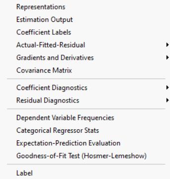
Dependent Variable Frequencies
This view displays a frequency and cumulative frequency table for the dependent variable in the binary model.
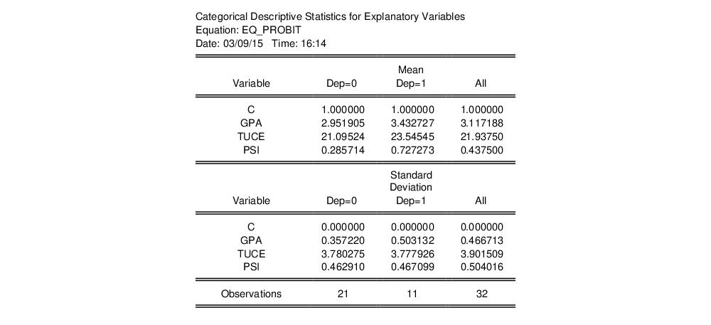
Categorical Regressor Stats
This view displays descriptive statistics (mean and standard deviation) for each regressor. The descriptive statistics are computed for the whole sample, as well as the sample broken down by the value of the dependent variable

:
Expectation-Prediction (Classification) Table
This view displays

tables of correct and incorrect classification based on a user specified prediction rule, and on expected value calculations. Click on . EViews opens a dialog prompting you to specify a prediction cutoff value,

, lying between zero and one. Each observation will be classified as having a predicted probability that lies above or below this cutoff.
After you enter the cutoff value and click on
OK, EViews will display four (bordered)

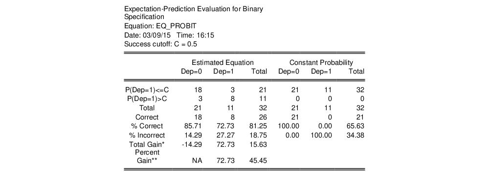
tables in the equation window. Each table corresponds to a contingency table of the predicted response classified against the observed dependent variable. The top two tables and associated statistics depict the classification results based upon the specified cutoff value:
In the left-hand table, we classify observations as having predicted probabilities
that are above or below the specified cutoff value (here set to the default of 0.5). In the upper right-hand table, we classify observations using

, the sample proportion of

observations. This probability, which is constant across individuals, is the value computed from estimating a model that includes only the intercept term, C.
“Correct” classifications are obtained when the predicted probability is less than or equal to the cutoff and the observed

, or when the predicted probability is greater than the cutoff and the observed

. In the example above, 18 of the Dep=0 observations and 8 of the Dep=1 observations are correctly classified by the estimated model.
It is worth noting that in the statistics literature, what we term the expectation-prediction table is sometimes referred to as the
classification table. The fraction of

observations that are correctly predicted is termed the
sensitivity, while the fraction of

observations that are correctly predicted is known as
specificity. In EViews, these two values, expressed in percentage terms, are labeled “% Correct”. Overall, the estimated model correctly predicts 81.25% of the observations (85.71% of the Dep=0 and 72.73% of the Dep=1 observations).
The gain in the number of correct predictions obtained in moving from the right table to the left table provides a measure of the predictive ability of your model. The gain measures are reported in both absolute percentage increases (
Total Gain), and as a percentage of the incorrect classifications in the constant probability model (
Percent Gain). In the example above, the restricted model predicts that all 21 individuals will have Dep=0. This prediction is correct for the 21

observations, but is incorrect for the 11

observations.
The estimated model improves on the Dep=1 predictions by 72.73 percentage points, but does more poorly on the Dep=0 predictions (-14.29 percentage points). Overall, the estimated equation is 15.62 percentage points better at predicting responses than the constant probability model. This change represents a 45.45 percent improvement over the 65.62 percent correct prediction of the default model.
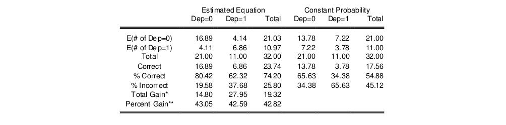
The bottom portion of the equation window contains analogous prediction results based upon expected value calculations:
In the left-hand table, we compute the expected number of

and

observations in the sample. For example,
E(# of Dep=0) is computed as:
 | (31.13) |
where the cumulative distribution function

is for the normal, logistic, or extreme value distribution.
In the lower right-hand table, we compute the expected number of

and

observations for a model estimated with only a constant. For this restricted model,
E(# of Dep=0) is computed as

, where

is the sample proportion of

observations. EViews also reports summary measures of the total gain and the percent (of the incorrect expectation) gain.
Among the 21 individuals with

, the expected number of

observations in the estimated model is 16.89. Among the 11 observations with

, the expected number of

observations is 6.86. These numbers represent roughly a 19.32 percentage point (42.82 percent) improvement over the constant probability model.
Goodness-of-Fit Tests
This view allows you to perform Pearson

-type tests of goodness-of-fit. EViews carries out two goodness-of-fit tests: Hosmer-Lemeshow (1989) and Andrews (1988a, 1988b). The idea underlying these tests is to compare the fitted expected values to the actual values
by group. If these differences are “large”, we reject the model as providing an insufficient fit to the data.
Details on the two tests are described in the
“Technical Notes”. Briefly, the tests differ in how the observations are grouped and in the asymptotic distribution of the test statistic. The Hosmer-Lemeshow test groups observations on the basis of the predicted probability that

. The Andrews test is a more general test that groups observations on the basis of any series or series expression.
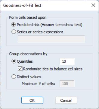
To carry out the test, select
You must first decide on the grouping variable. You can select Hosmer-Lemeshow (predicted probability) grouping by clicking on the corresponding radio button, or you can select series grouping, and provide a series to be used in forming the groups.
Next, you need to specify the grouping rule. EViews allows you to group on the basis of either distinct values or quantiles of the grouping variable.
If your grouping variable takes relatively few distinct values, you should choose the grouping. EViews will form a separate group for each distinct value of the grouping variable. For example, if your grouping variable is TUCE, EViews will create a group for each distinct TUCE value and compare the expected and actual numbers of

observations in each group. By default, EViews limits you to 100 distinct values. If the distinct values in your grouping series exceeds this value, EViews will return an error message. If you wish to evaluate the test for more than 100 values, you must explicitly increase the maximum number of distinct values.
If your grouping variable takes on a large number of distinct values, you should select , and enter the number of desired bins in the edit field. If you select this method, EViews will group your observations into the number of specified bins, on the basis of the ordered values of the grouping series. For example, if you choose to group by TUCE, select , and enter 10, EViews will form groups on the basis of TUCE deciles.
If you choose to group by quantiles and there are ties in the grouping variable, EViews may not be able to form the exact number of groups you specify unless tied values are assigned to different groups. Furthermore, the number of observations in each group may be very unbalanced. Selecting the randomize ties option randomly assigns ties to adjacent groups in order to balance the number of observations in each group.
Since the properties of the test statistics require that the number of observations in each group is “large”, some care needs to be taken in selecting a rule so that you do not end up with a large number of cells, each containing small numbers of observations.
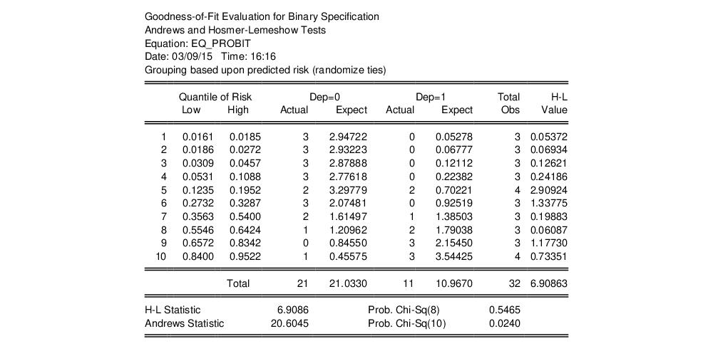
By default, EViews will perform the test using Hosmer-Lemeshow grouping. The default grouping method is to form deciles. The test result using the default specification is given by:
The columns labeled “Quantiles of Risk” depict the high and low value of the predicted probability for each decile. Also depicted are the actual and expected number of observations in each group, as well as the contribution of each group to the overall Hosmer-Lemeshow (H-L) statistic—large values indicate large differences between the actual and predicted values for that decile.
The

statistics are reported at the bottom of the table. Since grouping on the basis of the fitted values falls within the structure of an Andrews test, we report results for both the H-L and the Andrews test statistic. The
p-value for the HL test is large while the value for the Andrews test statistic is small, providing mixed evidence of problems. Furthermore, the relatively small sample sizes suggest that caution is in order in interpreting the results.
Procedures for Binary Equations
In addition to the usual procedures for equations, EViews allows you to forecast the dependent variable and linear index, or to compute a variety of residuals associated with the binary model.
Forecast
EViews allows you to compute either the fitted probability,
, or the fitted values of the index

. From the equation toolbar select , and then click on the desired entry.
As with other estimators, you can select a forecast sample, and display a graph of the forecast. If your explanatory variables,

, include lagged values of the binary dependent variable

, forecasting with the
Dynamic option instructs EViews to use the fitted values

, to derive the forecasts, in contrast with the
Static option, which uses the actual (lagged)

.
Neither forecast evaluations nor automatic calculation of standard errors of the forecast are currently available for this estimation method. The latter can be computed using the variance matrix of the coefficients obtained by displaying the covariance matrix view using or using the @covariance member function.
You can use the fitted index in a variety of ways, for example, to compute the marginal effects of the explanatory variables. Simply forecast the fitted index and save the results in a series, say XB. Then the auto-series
@dnorm(-xb),
@dlogistic(-xb), or
@dextreme(-xb) may be multiplied by the coefficients of interest to provide an estimate of the derivatives of the expected value of

with respect to the
j-th variable in

:
 | (31.14) |
Make Residual Series
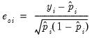
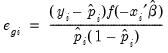
gives you the option of generating one of the following three types of residuals:
Ordinary | |
Standardized | |
Generalized | |
where
is the fitted probability, and the distribution and density functions

and

, depend on the specified distribution.
The ordinary residuals have been described above. The standardized residuals are simply the ordinary residuals divided by an estimate of the theoretical standard deviation. The generalized residuals are derived from the first order conditions that define the ML estimates. The first order conditions may be regarded as an orthogonality condition between the generalized residuals and the regressors

.
 | (31.15) |
This property is analogous to the orthogonality condition between the (ordinary) residuals and the regressors in linear regression models.
The usefulness of the generalized residuals derives from the fact that you can easily obtain the score vectors by multiplying the generalized residuals by each of the regressors in

. These scores can be used in a variety of LM specification tests (see Chesher, Lancaster and Irish (1985), and Gourieroux, Monfort, Renault, and Trognon (1987)). We provide an example below.
Demonstrations
You can easily use the results of a binary model in additional analysis. Here, we provide demonstrations of using EViews to plot a probability response curve and to test for heteroskedasticity in the residuals.
Plotting Probability Response Curves
You can use the estimated coefficients from a binary model to examine how the predicted probabilities vary with an independent variable. To do so, we will use the EViews built-in modeling features. (The following discussion skims over many of the useful features of EViews models. Those wishing greater detail should consult
“Models”.)
For the probit example above, suppose we are interested in the effect of teaching method (PSI) on educational improvement (GRADE). We wish to plot the fitted probabilities of GRADE improvement as a function of GPA for the two values of PSI, fixing the values of other variables at their sample means.
First, we create a model out of the estimated equation by selecting from the equation toolbar. EViews will create an untitled model object linked to the estimated equation and will open the model window.
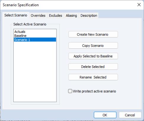
What we will do is to use the model to solve for values of the probabilities for various values of GPA, with TUCE equal to the mean value, and PSI equal to 0 in one case, and PSI equal to 1 in a second case. We will define scenarios in the model so that calculations are performed using the desired values. Click on the button on the model toolbar to display the dialog and click on to define the settings for that scenario.
The dialog allows us to define a set of assumptions under which we will solve the model. Click on the tab and enter “GPA PSI TUCE”. Defining these overrides tells EViews to use the values in the series GPA_1, PSI_1, and TUCE_1 instead of the original GPA, PSI, and TUCE when solving for GRADE under Scenario 1.
Having defined the first scenario, we must create the series GPA_1, PSI_1 and TUCE_1 in our workfile. We wish to use these series to evaluate the GRADE probabilities for various values of GPA holding TUCE equal to its mean value and PSI equal to 0.
First, we will use the command line to fill GPA_1 with a grid of values ranging from 2 to 4. The easiest way to do this is to use the @trend function:
series gpa_1 = 2+(4-2)*@trend/(@obs(@trend)-1)
Recall that @trend creates a series that begins at 0 in the first observation of the sample, and increases by 1 for each subsequent observation, up through @obs-1.
Next we create series TUCE_1 containing the mean values of TUCE and a series PSI_1 which we set to zero:
series tuce_1 = @mean(tuce)
series psi_1 = 0
Having prepared our data for the first scenario, we will now use the model object to define an alternate scenario where PSI=1. Return to the tab, select , then select as the , and as the . Copying Scenario 1 creates a new scenario, Scenario 2, that instructs EViews to use the values in the series GPA_2, PSI_2, and TUCE_2 when solving for GRADE. These values are initialized from the corresponding Scenario 1 series defined previously. We then set PSI_2 equal to 1 by issuing the command
series psi_2 = 1
We are now ready to solve the model under the two scenarios. Click on the button and set the solution scenario to and the solution scenario to . Be sure to click on the checkbox so that EViews knows to solve for both. You can safely ignore the remaining solution settings and simply click on .
EViews will report that your model has solved successfully and will place the solutions in the series GRADE_1 and GRADE_2, respectively. To display the results, select , and enter:
gpa_1 grade_1 grade_2
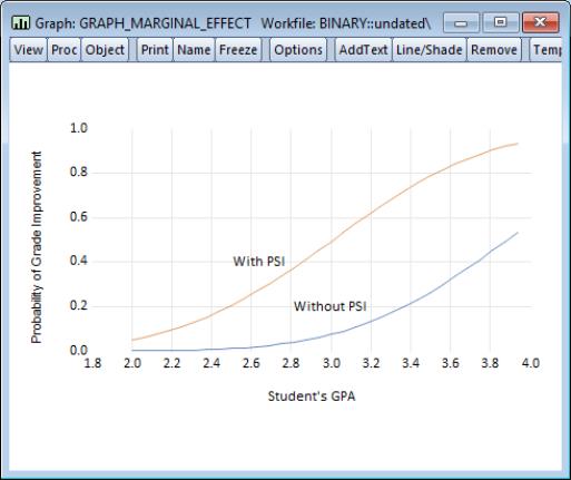
EViews will open an untitled group window containing these three series. Select to display a graph of the fitted GRADE probabilities plotted against GPA for those with PSI=0 (GRADE_1) and with PSI=1 (GRADE_2), both computed with TUCE evaluated at means.
We have annotated the graph slightly so that you can better judge the effect of the new teaching methods (PSI) on the probability of grade improvement for various values of the student’s GPA.
Testing for Heteroskedasticity
As an example of specification tests for binary dependent variable models, we carry out the LM test for heteroskedasticity using the artificial regression method described by Davidson and MacKinnon (1993, section 15.4). We test the null hypothesis of homoskedasticity against the alternative of heteroskedasticity of the form:
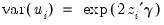 | (31.16) |
where

is an unknown parameter. In this example, we take PSI as the only variable in

. The test statistic is the explained sum of squares from the regression:
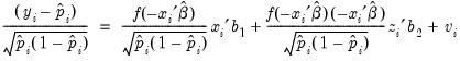 | (31.17) |
which is asymptotically distributed as a

with degrees of freedom equal to the number of variables in

(in this case 1).
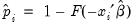
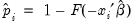
To carry out the test, we first retrieve the fitted probabilities

and fitted index

. Click on the button and first save the fitted probabilities as P_HAT and then the index as XB (you will have to click twice to save the two series).
Next, the dependent variable in the test regression may be obtained as the standardized residual. Select and select . We will save the series as BRMR_Y.
Lastly, we will use the built-in EViews functions for evaluating the normal density and cumulative distribution function to create a group object containing the independent variables:
series fac=@dnorm(-xb)/@sqrt(p_hat*(1-p_hat))
group brmr_x fac (gpa*fac) (tuce*fac) (psi*fac)
Then run the artificial regression by clicking on selecting Least Squares and entering:
brmr_y brmr_x (psi*(-xb)*fac)
You can obtain the fitted values by clicking on the button in the equation toolbar of this artificial regression. The LM test statistic is the sum of squares of these fitted values. If the fitted values from the artificial regression are saved in BRMR_YF, the test statistic can be saved as a scalar named LM_TEST:
scalar lm_test=@sumsq(brmr_yf)
which contains the value 1.5408. You can compare the value of this test statistic with the critical values from the chi-square table with one degree of freedom. To save the p-value as a scalar, enter the command:
scalar p_val=1-@cchisq(lm_test,1)
To examine the value of LM_TEST or P_VAL, double click on the name in the workfile window; the value will be displayed in the status line at the bottom of the EViews window. The p-value in this example is roughly 0.21, so we have little evidence against the null hypothesis of homoskedasticity.