Heckman Selection Model
The Heckman (1976) selection model, sometimes called the Heckit model, is a method for estimating regression models which suffer from sample selection bias. Under the Heckman selection framework, the dependent variable

is only observable for a portion of the data. A classic example, in economics, of the sample selection problem is the wage equation for women, whereby a woman’s wage is only observed if she makes the decision to enter the work place, and is unobservable if she does not. Heckman’s (1976) paper that introduced the Heckman Selection model worked on this very problem.
EViews provides an estimator for the simple linear Heckman Selection Model. This model is specified as:
 | (31.38) |
 | (31.39) |
where is

a binary variable, with

only observed when

.

and

are error terms which follow a bivariate normal distribution:
 | (31.40) |
with scale parameter

and correlation coefficient

. Note that we have normalized the variance of

to 1 since this variance is not identified in this model.
Equation
Equation (31.38) is generally referred to as the response equation, with

the variable of interest. Equation
Equation (31.39) is termed the selection equation and determines whether is

observed or not.
EViews offers two different methods of estimating this model: Heckman’s original two-step method and a Maximum Likelihood method.
The Heckman Two-Step Method
The Heckman two-step method is based around the observation that:
 | (31.41) |
where

is the Inverse Mills Ratio (Greene, 2008), and

and

are the standard normal density and cumulative distribution function, respectively. Then we may specify a regression model:
 | (31.42) |
The two-step method proceeds by first estimating a Probit regression for
Equation (31.39) to obtain an estimate of

, from which

may be calculated. A least squares regression of

on

and

 | (31.43) |
is then computed, yielding consistent estimates of

and

. An estimator for the error standard deviation

may be obtained from the usual standard error of the regression

, and the ratio estimator

follows.
The estimator of the coefficient covariance matrix of the two-step method is given by:
 | (31.44) |
where

,

is a diagonal matrix with

on the diagonals,

is an identity matrix,

, and

is the coefficient covariance matrix from the Probit estimation of
Equation (31.39).
Maximum Likelihood
The maximum likelihood method of estimating the Heckman Selection Model is performed using the log-likelihood function given by:
 | (31.45) |
where the first summation is over observations for which

(
i.e., when

is unobserved), and the second for observations for which

(
i.e., when

is observed).
It is straightforward to maximize this log-likelihood function with respect to the parameters,

. However, this maximization is unrestricted with regards to

and

, when, in fact, there are restrictions of the form

and

imposed on the parameters. EViews optimizes the model using transformed versions of the parameters:
 | (31.46) |
 | (31.47) |
to impose the restrictions.
Starting values for the optimization can be obtained using the Heckman two-step method outlined above.
As with most maximum likelihood estimations, the covariance matrix of the estimated parameters can be calculated as either

(where

is the Hessian matrix, the information matrix),

(where

is the matrix of gradients), or as

(the Huber/White matrix).
Estimating the Heckman Selection Model in EViews
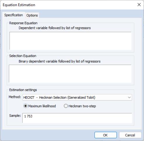
To estimate the Heckman Selection Model, open the equation dialog by selecting or in the main EViews menu and selecting from the dropdown menu. Alternately, you may enter the command heckit in the command line.
The first page of the dialog, the tab, lets you specify both the response equation
Equation (31.38) and the selection equation
Equation (31.39). Both equations should be specified as the dependent variable followed by a space delimited list of regressors. Note that the dependent variable for the selection equation should be series containing only zeros and ones.
The page also lets you select the type of estimation method by selecting one of the two radio buttons; either or .
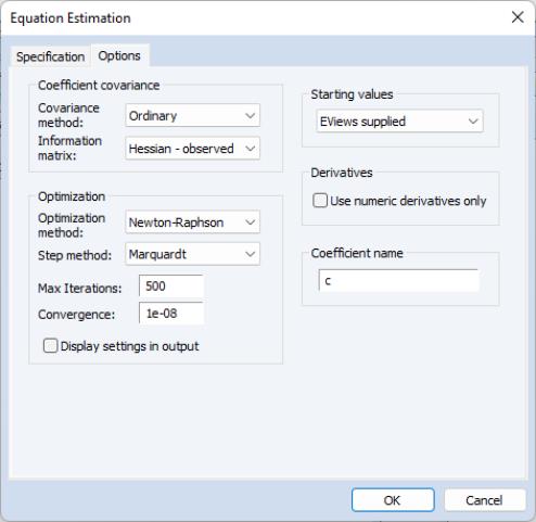
If you have chosen to estimate via maximum likelihood, the tab of the dialog lets you specify the type of covariance matrix, by using the dropdown menu. You may choose from , , and . You may also choose starting values for the maximum likelihood procedure. You may select to perform the Heckman two-step procedure to obtain starting values, or you can down-weight those starting values by choosing a multiple of them. The option will use the specified coefficient vector in the workfile to obtain starting values.
An Example
As an example of the estimation of the Heckman Selection model, we take one of the results from Econometric Analysis by William H. Greene (6th Edition, p. 888, Example 24.8), which uses data from the Mroz (1987) study of the labor supply of married women to estimate a wage equation for women. Only 428 of the 753 women studied participated in the labor force, so a selection equation is provided to model the sample selection behavior of married women.
The wage equation is given by:
 | (31.48) |
where EXPER is a measure of each woman’s experience, EDUC is her level of education, and CITY is a dummy variable for whether she lives in a city or not.
The selection equation is given by:
 | (31.49) |
where LFP is a binary variable taking a value of 1 if the woman is in the labor force, and 0 otherwise, AGE is her age, FAMINC is the level of household income not earned by the woman, and KIDS is a dummy variable for whether she has children.
You can bring the Mroz data directly into EViews from Greene’s website, using the following EViews command:
wfopen http://www.stern.nyu.edu/~wgreene/Text/Edition7/TableF5-1.txt
In this data, the wage data are in the series WW, experience is AX, education is in WE, the city dummy is CIT, labor force participation is LFP, age is WA, and family income is FAMINC. There is no kids dummy variable, but there are two variables containing the number of children below K6 education (KL6), and the number of kids between K6 education and 18 (K618). We can create the dummy variable simply by testing whether the sum of those two variables is greater than 0.
To estimate this equation in EViews, we click on …, and then change the equation method to . In the box we type:
ww c ax ax^2 we cit
And in the box we type:
lfp c wa wa^2 faminc we (kl6+k618)>0
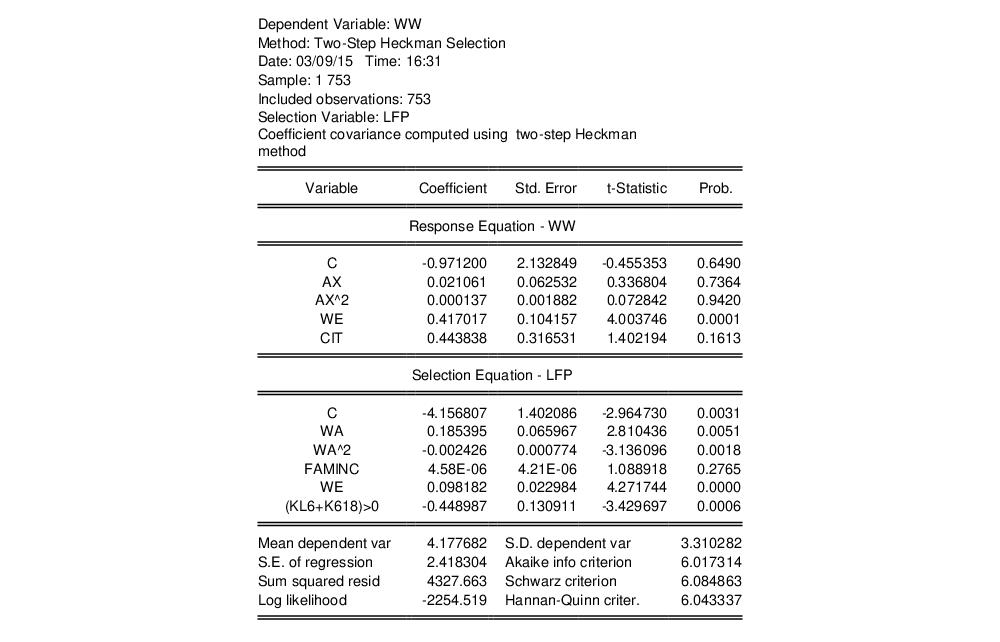
To begin we select the estimation method. After clicking , the estimation results show and replicate the results in the first pane of Table 24.3 in Greene (note that Greene only shows the estimates of the Wage equation, plus

and

).
We can modify our equation to use as the estimation method. Click on the button to bring up the estimation dialog and change the method to . Next,click on the tab and change the to and click on to estimate the equation. The results match the second pane of Table 24.3 in Greene.
 is only observable for a portion of the data. A classic example, in economics, of the sample selection problem is the wage equation for women, whereby a woman’s wage is only observed if she makes the decision to enter the work place, and is unobservable if she does not. Heckman’s (1976) paper that introduced the Heckman Selection model worked on this very problem.
 is only observable for a portion of the data. A classic example, in economics, of the sample selection problem is the wage equation for women, whereby a woman’s wage is only observed if she makes the decision to enter the work place, and is unobservable if she does not. Heckman’s (1976) paper that introduced the Heckman Selection model worked on this very problem.

 a binary variable, with
  only observed when
  .
.  and
and  are error terms which follow a bivariate normal distribution:
 and correlation coefficient
  . Note that we have normalized the variance of
  to 1 since this variance is not identified in this model.
 the variable of interest. Equation
 observed or not.
 is the Inverse Mills Ratio (Greene, 2008), and
  and
and  are the standard normal density and cumulative distribution function, respectively. Then we may specify a regression model:
 , from which
  may be calculated. A least squares regression of
  on
on  and
and 

 and
and  . An estimator for the error standard deviation
  may be obtained from the usual standard error of the regression
  , and the ratio estimator
  follows.
 ,
,  is a diagonal matrix with
  on the diagonals,
  is an identity matrix,
  , and
, and  is the coefficient covariance matrix from the Probit estimation of

 (
( is unobserved), and the second for observations for which
  (
( is observed).
 . However, this maximization is unrestricted with regards to
  and
and  , when, in fact, there are restrictions of the form
  and
and  imposed on the parameters. EViews optimizes the model using transformed versions of the parameters:

 (where
  is the Hessian matrix, the information matrix),
  (where
  is the matrix of gradients), or as
  (the Huber/White matrix).


 and
and  ).
).
