Examples
In this section, we provide extended examples of working with the logl object to estimate a multinomial logit and a maximum likelihood AR(1) specification. Example programs for these and several other specifications are provided in your default EViews data directory. If you set your default directory to point to the EViews data directory, you should be able to issue a RUN command for each of these programs to create the logl object and to estimate the unknown parameters.
Multinomial Logit (mlogit1.prg)
In this example, we demonstrate how to specify and estimate a simple multinomial logit model using the logl object. Suppose the dependent variable Y can take one of three categories 1, 2, and 3. Further suppose that there are data on two regressors, X1 and X2 that vary across observations (individuals). Standard examples include variables such as age and level of education. Then the multinomial logit model assumes that the probability of observing each category in Y is given by:
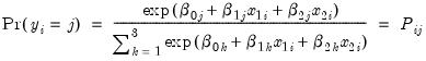 | (41.8) |
for

. Note that the parameters

are specific to each category so there are

parameters in this specification. The parameters are not all identified unless we impose a normalization, so we normalize the parameters of the first choice category

to be all zero:
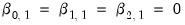
(see, for example, Greene (2008, Section 23.11.1).
The log likelihood function for the multinomial logit can be written as:
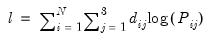 | (41.9) |
where

is a dummy variable that takes the value 1 if observation

has chosen alternative

and 0 otherwise. The first-order conditions are:
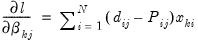 | (41.10) |
for

and

.
We have provided, in the Example Files subdirectory of your default EViews directory, a workfile “Mlogit.WK1” containing artificial multinomial data. The program begins by loading this workfile:
' load artificial data
%evworkfile = @evpath + "\example files\logl\mlogit"
load "{%evworkfile}"
from the EViews example directory.
Next, we declare the coefficient vectors that will contain the estimated parameters for each choice alternative:
' declare parameter vector
coef(3) b2
coef(3) b3
As an alternative, we could have used the default coefficient vector C.
We then set up the likelihood function by issuing a series of append statements:
mlogit.append xb2 = b2(1)+b2(2)*x1+b2(3)*x2
mlogit.append xb3 = b3(1)+b3(2)*x1+b3(3)*x2
' define prob for each choice
mlogit.append denom = 1+exp(xb2)+exp(xb3)
mlogit.append pr1 = 1/denom
mlogit.append pr2 = exp(xb2)/denom
mlogit.append pr3 = exp(xb3)/denom
' specify likelihood
mlogit.append logl1 = (1-dd2-dd3)*log(pr1) +dd2*log(pr2)+dd3*log(pr3)
Since the analytic derivatives for the multinomial logit are particularly simple, we also specify the expressions for the analytic derivatives to be used during estimation and the appropriate @deriv statements:
' specify analytic derivatives
for!i = 2 to 3
mlogit.append @deriv b{!i}(1) grad{!i}1 b{!i}(2) grad{!i}2 b{!i}(3) grad{!i}3
mlogit.append grad{!i}1 = dd{!i}-pr{!i}
mlogit.append grad{!i}2 = grad{!i}1*x1
mlogit.append grad{!i}3 = grad{!i}1*x2
next
Note that if you were to specify this likelihood interactively, you would simply type the expression that follows each append statement directly into the MLOGIT object.
This concludes the actual specification of the likelihood object. Before estimating the model, we get the starting values by estimating a series of binary logit models:
' get starting values from binomial logit
equation eq2.binary(d=l) dd2 c x1 x2
b2 = eq2.@coefs
equation eq3.binary(d=l) dd3 c x1 x2
b3 = eq3.@coefs
To check whether you have specified the analytic derivatives correctly, choose or use the command:
show mlogit.checkderiv
If you have correctly specified the analytic derivatives, they should be fairly close to the numeric derivatives.
We are now ready to estimate the model. Either click the button or use the command:
' do MLE
mlogit.ml(showopts, m=1000, c=1e-5)
show mlogit.output
Note that you can examine the derivatives for this model using the view, or you can examine the series in the workfile containing the gradients. You can also look at the intermediate results and log likelihood values. For example, to look at the likelihood contributions for each individual, simply double click on the LOGL1 series.
AR(1) Model (ar1.prg)
In this example, we demonstrate using the logl to compute full maximum likelihood estimates of an AR(1). This logl example replicates the ML estimator that is built-into the least squares estimator for an equation (
“Time Series Regression”).
To illustrate, we first generate data that follows an AR(1) process:
' make up data
create m 80 89
rndseed 123
series y=0
smpl @first+1 @last
y = 1+0.85*y(-1) + nrnd
The exact Gaussian likelihood function for an AR(1) model is given by:
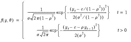 | (41.11) |
where

is the constant term,

is the AR(1) coefficient, and

is the error variance, all to be estimated (see for example Hamilton, 1994, Chapter 5.2).
Since the likelihood function evaluation differs for the first observation in our sample, we create a dummy variable indicator for the first observation:
' create dummy variable for first obs
series d1 = 0
smpl @first @first
d1 = 1
smpl @all
Next, we declare the coefficient vectors to store the parameter estimates and initialize them with the least squares estimates:
' set starting values to LS (drops first obs)
equation eq1.ls y c ar(1)
coef(1) rho = c(2)
coef(1) s2 = eq1.@se^2
We then specify the likelihood function. We make use of the @recode function to differentiate the evaluation of the likelihood for the first observation from the remaining observations. Note: the @recode function used here uses the updated syntax for this function—please double-check the current documentation for details.
' set up likelihood
logl ar1
ar1.append @logl logl1
ar1.append var = @recode(d1=1,s2(1)/(1-rho(1)^2),s2(1))
ar1.append res = @recode(d1=1,y-c(1)/(1-rho(1)),y-c(1)-rho(1)*y(-1))
ar1.append sres = res/@sqrt(var)
ar1.append logl1 = log(@dnorm(sres))-log(var)/2
The likelihood specification uses the built-in function @dnorm for the standard normal density. The second term is the Jacobian term that arises from transforming the standard normal variable to one with non-unit variance. (You could, of course, write out the likelihood for the normal distribution without using the @dnorm function.)
The program displays the MLE together with the least squares estimates:
' do MLE
ar1.ml(showopts, m=1000, c=1e-5)
show ar1.output
' compare with EViews AR(1) which ignores first obs
show eq1.output
Additional Examples
The following additional example programs can be found in the “Example Files” subdirectory of your default EViews directory.
• (clogit1.prg): estimates a conditional logit with 3 outcomes and both individual specific and choice specific regressors. The program also displays the prediction table and carries out a Hausman test for independence of irrelevant alternatives (IIA). See Greene (2008, Chapter 23.11.1) for a discussion of multinomial logit models.
• (boxcox1.prg): estimates a simple bivariate regression with an estimated Box-Cox transformation on both the dependent and independent variables. Box-Cox transformation models are notoriously difficult to estimate and the results are very sensitive to starting values.
• (diseq1.prg): estimates the switching model in exercise 15.14–15.15 of Judge et al. (1985, p. 644–646). Note that there are some typos in Judge et al. (1985, p. 639–640). The program uses the likelihood specification in Quandt (1988, page 32, equations 2.3.16–2.3.17).
• (hetero1.prg): estimates a linear regression model with multiplicative heteroskedasticity.
• y (hprobit1.prg): estimates a probit specification with multiplicative heteroskedasticity.
• (gprobit1.prg): estimates a probit with grouped data (proportions data).
• (nlogit1.prg): estimates a nested logit model with 2 branches. Tests the IIA assumption by a Wald test. See Greene (2008, Chapter 23.11.4) for a discussion of nested logit models.
• (zpoiss1.prg): estimates the zero-altered Poisson model. Also carries out the non-nested LR test of Vuong (1989). See Greene (2008, Chapter 25.4) for a discussion of zero-altered Poisson models and Vuong’s non-nested likelihood ratio test.
• (heckman1.prg): estimates Heckman’s two equation sample selection model by MLE using the two-step estimates as starting values.
• (weibull1.prg): estimates the uncensored Weibull hazard model described in Greene (2008, example 25.4).
• (arch_t1.prg): estimates a GARCH(1,1) model with
t-distribution. The log likelihood function for this model can be found in Hamilton (1994, equation 21.1.24, page 662). Note that this model may more easily be estimated using the standard ARCH estimation tools provided in EViews (
“ARCH and GARCH Estimation”).
• (garch1.prg): estimates an MA(1)-GARCH(1,1) model with coefficient restrictions in the conditional variance equation. This model is estimated by Bollerslev, Engle, and Nelson (1994, equation 9.1, page 3015) for different data.
• (egarch1.prg): estimates Nelson’s (1991) exponential GARCH with generalized error distribution. The specification and likelihood are described in Hamilton (1994, p. 668–669). Note that this model may more easily be estimated using the standard ARCH estimation tools provided in EViews (
“ARCH and GARCH Estimation”).
• (bv_garch.prg and tv_garch.prg): estimates the bi- or the tri-variate version of the BEKK GARCH specification (Engle and Kroner, 1995). Note that this specification may be estimated using the built-in procedures available in the system object (
“System Estimation”).