Specification
To create a likelihood object, choose or type the keyword logl in the command window. The likelihood window will open with a blank specification view. The specification view is a text window into which you enter a list of statements which describe your statistical model, and in which you set options which control various aspects of the estimation procedure.
Specifying the Likelihood
As described in the overview above, the core of the likelihood specification is a set of assignment statements which, when evaluated, generate a series containing the log likelihood contribution of each observation in the sample. There can be as many or as few of these assignment statements as you wish.
Each likelihood specification must contain a control statement which provides the name of the series which is used to contain the likelihood contributions. The format of this statement is:
@logl series_name
where series_name is the name of the series which will contain the contributions. This control statement may appear anywhere in the logl specification.
Whenever the specification is evaluated, whether for estimation or for carrying out a View or Proc, each assignment statement will be evaluated at the current parameter values, and the results stored in a series with the specified name. If the series does not exist, it will be created automatically. If the series already exists, EViews will use the existing series for storage, and will overwrite the data contained in the series.
If you would like to remove one or more of the series used in the specification after evaluation, you can use the @temp statement, as in:
@temp series_name1 series_name2
This statement tells EViews to delete any series in the list after evaluation of the specification is completed. Deleting these series may be useful if your logl creates a lot of intermediate results, and you do not want the series containing these results to clutter your workfile.
Parameter Names
In the example above, we used the coefficients C(1) to C(5) as names for our unknown parameters. More generally, any element of a named coefficient vector which appears in the specification will be treated as a parameter to be estimated.
In the conditional heteroskedasticity example, you might choose to use coefficients from three different coefficient vectors: one vector for the mean equation, one for the variance equation, and one for the variance parameters. You would first create three named coefficient vectors by the commands:
coef(3) beta
coef(1) scale
coef(1) alpha
You could then write the likelihood specification as:
@logl logl1
res = y - beta(1) - beta(2)*x - beta(3)*z
var = scale(1)*z^alpha(1)
logl1 = log(@dnorm(res/@sqrt(var))) - log(var)/2
Since all elements of named coefficient vectors in the specification will be treated as parameters, you should make certain that all coefficients really do affect the value of one or more of the likelihood contributions. If a parameter has no effect upon the likelihood, you will experience a singularity error when you attempt to estimate the parameters.
Note that all objects other than coefficient elements will be considered fixed and will not be updated during estimation. For example, suppose that SIGMA is a named scalar in your workfile. Then if you redefine the subexpression for VAR as:
var = sigma*z^alpha(1)
EViews will not estimate SIGMA. The value of SIGMA will remain fixed at its value at the start of estimation.
Order of Evaluation
The logl specification contains one or more assignment statements which generate the series containing the likelihood contributions. EViews always evaluates from top to bottom when executing these assignment statements, so expressions which are used in subsequent calculations should always be placed first.
EViews must also iterate through the observations in the sample. Since EViews iterates through both the equations in the specification and the observations in the sample, you will need to specify the order in which the evaluation of observations and equations occurs.
By default, EViews evaluates the specification by observation so that all of the assignment statements are evaluated for the first observation, then for the second observation, and so on across all the observations in the estimation sample. This is the correct order for recursive models where the likelihood of an observation depends on previously observed (lagged) values, as in AR or ARCH models.
You can change the order of evaluation so EViews evaluates the specification by equation, so the first assignment statement is evaluated for all the observations, then the second assignment statement is evaluated for all the observations, and so on for each of the assignment statements in the specification. This is the correct order for models where aggregate statistics from intermediate series are used as input to subsequent calculations.
You can control the method of evaluation by adding a statement to the likelihood specification. To force evaluation by equation, simply add a line containing the keyword “@byeqn”. To explicitly state that you require evaluation by observation, the “@byobs” keyword can be used. If no keyword is provided, @byobs is assumed.
In the conditional heteroskedasticity example above, it does not matter whether the assignment statements are evaluated by equation (line by line) or by observation, since the results do not depend upon the order of evaluation.
However, if the specification has a recursive structure, or if the specification requires the calculation of aggregate statistics based on intermediate series, you must select the appropriate evaluation order if the calculations are to be carried out correctly.
As an example of the @byeqn statement, consider the following specification:
@logl robust1
@byeqn
res1 = y-c(1)-c(2)*x
delta = @abs(res1)/6/@median(@abs(res1))
weight = (delta<1)*(1-delta^2)^2
robust1 = -(weight*res1^2)
This specification performs robust regression by downweighting outlier residuals at each iteration. The assignment statement for delta computes the median of the absolute value of the residuals in each iteration, and this is used as a reference point for forming a weighting function for outliers. The @byeqn statement instructs EViews to compute all residuals RES1 at a given iteration before computing the median of those residuals when calculating the DELTA series.
Analytic Derivatives
By default, when maximizing the likelihood and forming estimates of the standard errors, EViews computes numeric derivatives of the likelihood function with respect to the parameters. If you would like to specify an analytic expression for one or more of the derivatives, you may use the @deriv statement. The @deriv statement has the form:
@deriv pname1 sname1 pname2 sname2 …
where pname is a parameter in the model and sname is the name of the corresponding derivative series generated by the specification.
For example, consider the following likelihood object that specifies a multinomial logit model:
' multinomial logit with 3 outcomes
@logl logl1
xb2 = b2(1)+b2(2)*x1+b2(3)*x2
xb3 = b3(1)+b3(2)*x1+b3(3)*x2
denom = 1+exp(xb2)+exp(xb3)
' derivatives wrt the 2nd outcome params
@deriv b2(1) grad21 b2(2) grad22 b2(3) grad23
grad21 = d2-exp(xb2)/denom
grad22 = grad21*x1
grad23 = grad21*x2
' derivatives wrt the 3rd outcome params
@deriv b3(1) grad31 b3(2) grad32 b3(3) grad33
grad31 = d3-exp(xb3)/denom
grad32 = grad31*x1
grad33 = grad31*x2
' specify log likelihood
logl1 = d2*xb2+d3*xb3-log(1+exp(xb2)+exp(xb3))
See Greene (2008), Chapter 23.11.1 for a discussion of multinomial logit models. There are three possible outcomes, and the parameters of the three regressors (X1, X2 and the constant) are normalized relative to the first outcome. The analytic derivatives are particularly simple for the multinomial logit model and the two @deriv statements in the specification instruct EViews to use the expressions for GRAD21, GRAD22, GRAD23, GRAD31, GRAD32, and GRAD33, instead of computing numeric derivatives.
When working with analytic derivatives, you may wish to check the validity of your expressions for the derivatives by comparing them with numerically computed derivatives. EViews provides you with tools which will perform this comparison at the current values of parameters or at the specified starting values. See the discussion of the view of the likelihood object in
“Check Derivatives”.
Derivative Step Sizes
If analytic derivatives are not specified for any of your parameters, EViews numerically evaluates the derivatives of the likelihood function for those parameters. The step sizes used in computing the derivatives are controlled by two parameters:

(relative step size) and m (minimum step size). Let

denote the value of the parameter

at iteration

. Then the step size at iteration

is determined by:
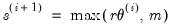 | (41.5) |
The two-sided numeric derivative is evaluated as:
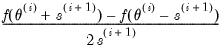 | (41.6) |
The one-sided numeric derivative is evaluated as:
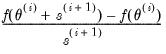 | (41.7) |
where

is the likelihood function. Two-sided derivatives are more accurate, but require roughly twice as many evaluations of the likelihood function and so take about twice as long to evaluate.
The @derivstep statement can be used to control the step size and method used to evaluate the derivative at each iteration. The @derivstep keyword should be followed by sets of three arguments: the name of the parameter to be set (or the keyword @all), the relative step size, and the minimum step size.
The default setting is (approximately):
@derivstep(1) @all 1.49e-8 1e-10
where “
1” in the parentheses indicates that one-sided numeric derivatives should be used and
@all indicates that the following setting applies to all of the parameters. The first number following
@all is the relative step size and the second number is the minimum step size. The default relative step size is set to the square root of machine epsilon

and the minimum step size is set to

.
The step size can be set separately for each parameter in a single or in multiple @derivstep statements. The evaluation method option specified in parentheses is a global option; it cannot be specified separately for each parameter.
For example, if you include the line:
@derivstep(2) c(2) 1e-7 1e-10
the relative step size for coefficient C(2) will be increased to

and a two-sided derivative will be used to evaluate the derivative. In a more complex example,
@derivstep(2) @all 1.49e-8 1e-10 c(2) 1e-7 1e-10 c(3) 1e-5 1e-8
computes two-sided derivatives using the default step sizes for all coefficients except C(2) and C(3). The values for these latter coefficients are specified directly.