Pooled Estimation
EViews pool objects allow you to estimate your model using least squares or instrumental variables (two-stage least squares), with correction for fixed or random effects in both the cross-section and period dimensions, AR errors, GLS weighting, and robust standard errors, all without rearranging or reordering your data.
We begin our discussion by walking you through the steps that you will take in estimating a pool equation. The wide range of models that EViews supports means that we cannot exhaustively describe all of the settings and specifications. A brief background discussion of the supported techniques is provided in
“Estimation Background”.
Estimating a Pool Equation
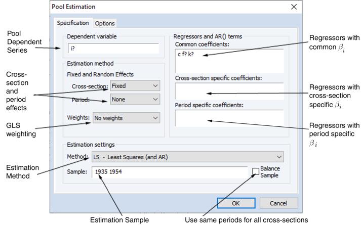
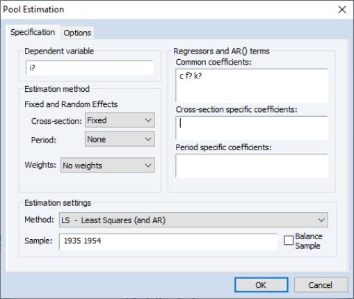
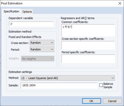
To estimate a pool equation specification, simply press the button on your pool object toolbar or select from the pool menu, and the basic pool estimation dialog will open:
First, you should specify the estimation settings in the lower portion of the dialog. Using the dropdown menu, you may choose between ordinary least squares regression, , two-stage least squares (instrumental variable) regression. If you select the latter, the dialog will differ slightly from this example, with the provision of an additional tab (page) for you to specify your instruments (see
“Instruments”).
You should also provide an estimation sample in the edit box. By default, EViews will use the specified sample string to form use the largest sample possible in each cross-section. An observation will be excluded if any of the explanatory or dependent variables for that cross-section are unavailable in that period.
The checkbox for Balanced Sample instructs EViews to perform listwise exclusion over all cross-sections. EViews will eliminate an observation if data are unavailable for any cross-section in that period. This exclusion ensures that estimates for each cross-section will be based on a common set of dates.
Note that if all of the observations for a cross-section unit are not available, that unit will temporarily be removed from the pool for purposes of estimation. The EViews output will inform you if any cross-section were dropped from the estimation sample.
You may now proceed to fill out the remainder of the dialog.
Dependent Variable
List a pool variable, or an EViews expression containing ordinary and pool variables, in the edit box.
Regressors and AR terms
On the right-hand side of the dialog, you should list your regressors in the appropriate edit boxes:
• Common coefficients: — enter variables that have the same coefficient across all cross-section members of the pool. EViews will include a single coefficient for each variable, and will label the output using the original expression.
• Cross-section specific coefficients: — list variables with different coefficients for each member of the pool. EViews will include a different coefficient for each cross-sectional unit, and will label the output using a combination of the cross-section identifier and the series name.
• Period specific coefficients: — list variables with different coefficients for each observed period. EViews will include a different coefficient for each period unit, and will label the output using a combination of the period identifier and the series name.
For example, if you include the ordinary variable TIME and POP? in the common coefficient list, the output will include estimates for TIME and POP?. If you include these variables in the cross-section specific list, the output will include coefficients labeled “_USA—TIME”, “_UK—TIME”, and “_USA—POP_USA”, “_UK—POP_UK”, etc.
Be aware that estimating your model with cross-section or period specific variables may generate large numbers of coefficients. If there are cross-section specific regressors, the number of these coefficients equals the product of the number of pool identifiers and the number of variables in the list; if there are period specific regressors, the number of corresponding coefficients is the number of periods times the number of variables in the list.
You may include AR terms in either the common or cross-section coefficients lists. If the terms are entered in the common coefficients list, EViews will estimate the model assuming a common AR error. If the AR terms are entered in the cross-section specific list, EViews will estimate separate AR terms for each pool member. See
“Specifying AR Terms” for a description of AR specifications.
Note that EViews only allows specification by list for pool equations. If you wish to estimate a nonlinear specification, you must first create a system object, and then edit the system specification (see
“Making a System”).
Fixed and Random Effects
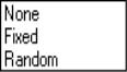
You should account for individual and period effects using the dropdown menus. By default, EViews assumes that there are no effects so that the dropdown menus are both set to . You may change the default settings to allow for either or effects in either the cross-section or period dimension, or both.
There are some specifications that are not currently supported. You may not, for example, estimate random effects models with cross-section specific coefficients, AR terms, or weighting. Furthermore, while two-way random effects specifications are supported for balanced data, they may not be estimated in unbalanced designs.
Note that when you select a fixed or random effects specification, EViews will automatically add a constant to the common coefficients portion of the specification if necessary, to ensure that the observation weighted sum of the effects is equal to zero.
Weights
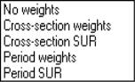
By default, all observations are given equal weight in estimation. You may instruct EViews to estimate your specification with estimated GLS weights using the dropdown menu labeled .
If you select , EViews will estimate a feasible GLS specification assuming the presence of cross-section heteroskedasticity. If you select , EViews estimates a feasible GLS specification correcting for both cross-section heteroskedasticity and contemporaneous correlation. Similarly, allows for period heteroskedasticity, while corrects for both period heteroskedasticity and general correlation of observations within a given cross-section. Note that the SUR specifications are each examples of what is sometimes referred to as the Parks estimator.
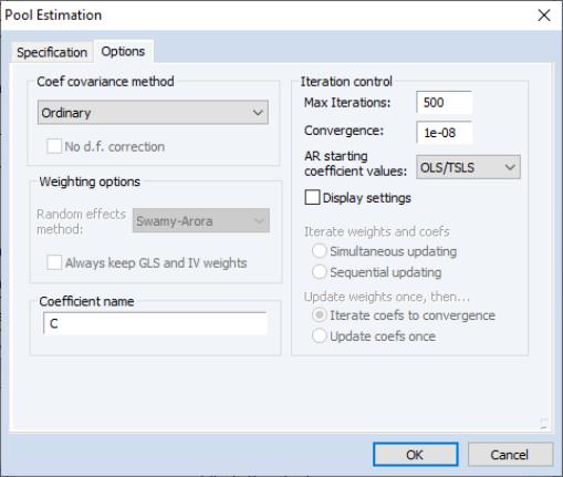
Options
Clicking on the tab in the dialog brings up a page displaying a variety of estimation options for pool estimation. Settings that are not currently applicable will be grayed out.
Coef Covariance Method
By default, EViews reports conventional estimates of coefficient standard errors and covariances.
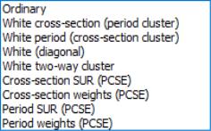
You may use the dropdown menu at the top of the page to select from the various robust methods available for computing the coefficient standard errors. The covariance calculations may be chosen to be robust under various assumptions, for example, general correlation of observations within a cross-section, or perhaps cross-section heteroskedasticity. Select for one-way period clustering, for one-way cross-section clustering, for unstructured heteroskedasticity robust covariances, or for clustering by both cross-section and period. Each of the methods is described in greater detail in
“Robust Coefficient Covariances”.
Note that the checkbox permits to you compute robust covariances without the leading degree of freedom correction term. This option may make it easier to match EViews results to those from other sources.
Weighting Options
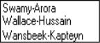
If you are estimating a specification that includes a random effects specification, EViews will provide you with a dropdown menu so that you may specify one of the methods for calculating estimates of the component variances. You may choose between the default , or methods. See
“Random Effects” for discussion of the differences between the methods. Note that the default Swamy-Arora method should be the most familiar from textbook discussions.
Details on these methods are provided in Baltagi (2005), Baltagi and Chang (1994), Wansbeek and Kapteyn (1989).
The checkbox labeled may be selected to require EViews to save all estimated GLS weights with the equation, regardless of their size. By default, EViews will not save estimated weights in system (SUR) settings, since the size of the required matrix may be quite large. If the weights are not saved with the equation, there may be some pool views and procedures that are not available.
Coefficient Name
By default, EViews uses the default coefficient vector C to hold the estimates of the coefficients and effects. If you wish to change the default, simply enter a name in the edit field. If the specified coefficient object exists, it will be used, after resizing if necessary. If the object does not exist, it will be created with the appropriate size. If the object exists but is an incompatible type, EViews will generate an error.
Iteration Control
The familiar and criterion edit boxes that allow you to set the convergence test for the coefficients and GLS weights.
If your specification contains AR terms, the dropdown menu allows you to specify starting values as a fraction of the OLS (with no AR) coefficients, zero, or user-specified values.
If is checked, EViews will display additional information about convergence settings and initial coefficient values (where relevant) at the top of the regression output.
The last set of radio buttons is used to determine the iteration settings for coefficients and GLS weighting matrices.
The first two settings, and should be employed when you want to ensure that both coefficients and weighting matrices are iterated to convergence. If you select the first option, EViews will, at every iteration, update both the coefficient vector and the GLS weights; with the second option, the coefficient vector will be iterated to convergence, then the weights will be updated, then the coefficient vector will be iterated, and so forth. Note that the two settings are identical for GLS models without AR terms.
If you select one of the remaining two cases, and , the GLS weights will only be updated once. In both settings, the coefficients are first iterated to convergence, if necessary, in a model with no weights, and then the weights are computed using these first-stage coefficient estimates. If the first option is selected, EViews will then iterate the coefficients to convergence in a model that uses the first-stage weight estimates. If the second option is selected, the first-stage coefficients will only be iterated once. Note again that the two settings are identical for GLS models without AR terms.
By default, EViews will update GLS weights once, and then will update the coefficients to convergence.
Instruments
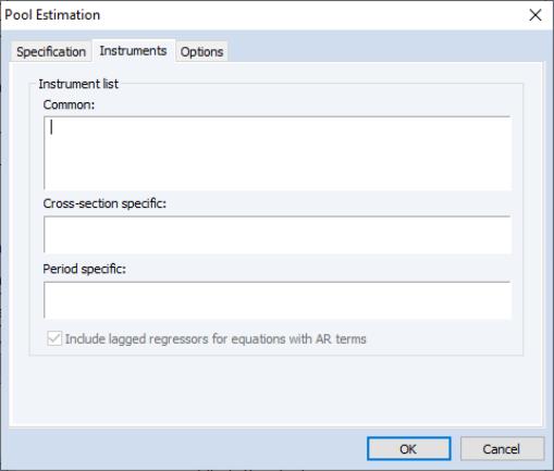
To estimate a pool specification using instrumental variables techniques, you should select in the dropdown menu at the bottom of the main () dialog page. EViews will respond by creating a three-tab dialog in which the middle tab (page) is used to specify your instruments.
As with the regression specification, the instrument list specification is divided into a set of , , and instruments. The interpretation of these lists is the same as for the regressors; if there are cross-section specific instruments, the number of these instruments equals the product of the number of pool identifiers and the number of variables in the list; if there are period specific instruments, the number of corresponding instruments is the number of periods times the number of variables in the list.
Note that you need not specify constant terms explicitly since EViews will internally add constants to the lists corresponding to the specification in the main page.
Lastly, there is a checkbox labeled that will be displayed if your specification includes AR terms. Recall that when estimating an AR specification, EViews performs nonlinear least squares on an AR differenced specification. By default, EViews will add lagged values of the dependent and independent regressors to the corresponding lists of instrumental variables to account for the modified differenced specification. If, however, you desire greater control over the set of instruments, you may uncheck this setting.
Pool Equation Examples
For illustrative purposes, we employ the balanced firm-level data from Grunfeld (1958) that have been used extensively as an example dataset (e.g., Baltagi, 2005). The workfile (“Grunfeld_Baltagi_pool.WF1”) contains annual observations on investment (I?), firm value (F?), and capital stock (K?) for 10 large U.S. manufacturing firms for the 20 years from 1935-54.
The pool identifiers for our data are “AR”, “CH”, “DM”, “GE”, “GM”, “GY”, “IB”, “UO”, “US”, “WH”.
We obviously cannot demonstrate all of the specifications that may be estimated using these data, but we provide a few illustrative examples.
Fixed Effects
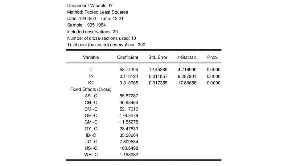
First, we estimate a model regressing I? on the common regressors F? and K?, with a cross-section fixed effect. All regression coefficients are restricted to be the same across all cross-sections, so this is equivalent to estimating a model on the stacked data, using the cross-sectional identifiers only for the fixed effect.
The top portion of the output from this regression, which shows the dependent variable, method, estimation and sample information is given by:
EViews displays both the estimates of the coefficients and the fixed effects. Note that EViews automatically includes a constant term so that the fixed effects estimates sum to zero and should be interpreted as deviations from an overall mean.
Note also that the estimates of the fixed effects do not have reported standard errors since EViews treats them as nuisance parameters for the purposes of estimation. If you wish to compute standard errors for the cross-section effects, you may estimate a model without a constant and explicitly enter the C in the Cross-section specific coefficients edit field.
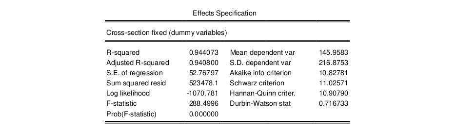
The bottom portion of the output displays the effects specification and summary statistics for the estimated model.
A few of these summary statistics require discussion. First, the reported R-squared and F-statistics are based on the difference between the residuals sums of squares from the estimated model, and the sums of squares from a single constant-only specification, not from a fixed-effect-only specification. As a result, the interpretation of these statistics is that they describe the explanatory power of the entire specification, including the estimated fixed effects. Second, the reported information criteria use, as the number of parameters, the number of estimated coefficients, including fixed effects. Lastly, the reported Durbin-Watson stat is formed simply by computing the first-order residual correlation on the stacked set of residuals.
Robust Standard Errors
We may reestimate this specification using White cross-section standard errors to allow for general contemporaneous correlation between the firm residuals. The “cross-section” designation is used to indicate that non-zero covariances are allowed across cross-sections (clustering by period). Simply click on the tab and select as the coefficient covariance matrix, then reestimate the model. The relevant portion of the output is given by:
The new output shows the method used for computing the standard errors, and the new standard error estimates, t-statistic values, and probabilities reflecting the robust calculation of the coefficient covariances.
Alternatively, we may adopt the Arellano (1987) approach of computing White coefficient covariance estimates that are robust to arbitrary within cross-section residual correlation (clustering by cross-section). Select the page and choose as the coefficient covariance method. The coefficient results are given by.
We caution that the White period results assume that the number of cross-sections is large, which is not the case in this example. In fact, the resulting coefficient covariance matrix is of reduced rank, a fact that EViews notes in the output.
AR Estimation
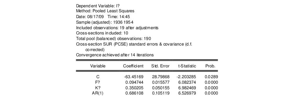
We may add an AR(1) term to the specification, and compute estimates using Cross-section SUR PCSE methods to compute standard errors that are robust to more contemporaneous correlation. EViews will estimate the transformed model using nonlinear least squares, will form an estimate of the residual covariance matrix, and will use the estimate in forming standard errors. The top portion of the results is given by:
Note in particular the description of the sample adjustment where we show that the estimation drops one observation for each cross-section when performing the AR differencing, as well as the description of the method used to compute coefficient covariances.
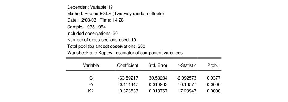
Random Effects
Alternatively, we may produce estimates for the two way random effects specification. First, in the page, we set both the cross-section and period effects dropdown menus to . Note that the dialog changes to show that weighted estimation is not available with random effects (nor is AR estimation).
Next, in the page we estimate the coefficient covariance using the method and we change the to use the method of computing the estimates of the random component variances.
Lastly, we click on to estimate the model.
The top portion of the dialog displays basic information about the specification, including the method used to compute the component variances, as well as the coefficient estimates and associated statistics:
The middle portion of the output (not depicted) displays the best-linear unbiased predictor estimates of the random effects themselves.
The next portion of the output describes the estimates of the component variances:
Here, we see that the estimated cross-section, period, and idiosyncratic error component standard deviations are 89.26, 15.78, and 51.72, respectively. As seen from the values of Rho, these components comprise 0.73, 0.02 and 0.25 of the total variance. Taking the cross-section component, for example, Rho is computed as:
 | (53.1) |
In addition, EViews reports summary statistics for the random effects GLS weighted data used in estimation, and a subset of statistics computed for the unweighted data.
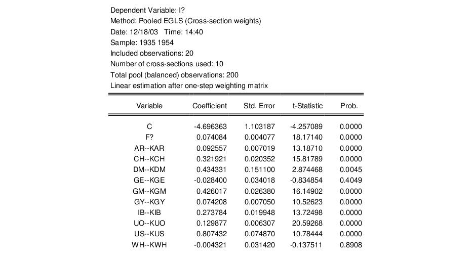
Cross-section Specific Regressors
Suppose instead that we elect to estimate a specification with I? as the dependent variable, C and F? as the common regressors, and K? as the cross-section specific regressor, using cross-section weighted least squares. The top portion of the output is given by:
Note that EViews displays results for each of the cross-section specific K? series, labeled using the equation identifier followed by the series name. For example, the coefficient labeled “AR--KAR” is the coefficient of KAR in the cross-section equation for firm AR.
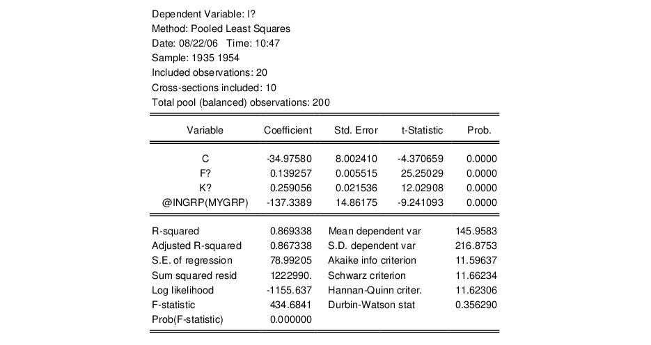
Group Dummy Variables
In our last example, we consider the use of the @INGRP pool function to estimate an specification containing group dummy variables (see
“Pool Series”). Suppose we modify our pool definition so that we have defined a group named “MYGROUP” containing the identifiers “GE”, “GM”, and “GY”. We may then estimate a pool specification using the common regressor list:
c f? k? @ingrp(mygrp)
where the latter pool series expression refers to a set of 10 implicit series containing dummy variables for group membership. The implicit series associated with the identifiers “GE”, “GM”, and “GY” will contain the value 1, and the remaining seven series will contain the value 0.
The results from this estimation are given by:
We see that the mean value of I? for the three groups is substantially lower than for the remaining groups, and that the difference is statistically significant at conventional levels.
Pool Equation Views and Procedures
Once you have estimated your pool equation, you may examine your output in the usual ways:
Representation
Select to examine your specification. EViews estimates your pool as a system of equations, one for each cross-section unit.
Estimation Output
will change the display to show the results from the pooled estimation.
As with other estimation objects, you can examine the estimates of the coefficient covariance matrix by selecting .
Testing
EViews allows you to perform coefficient tests on the estimated parameters of your pool equation. Select and enter the restriction to be tested. Additional tests are described in the panel discussion
“Panel Equation Testing”Residuals
You can view your residuals in spreadsheet or graphical format by selecting or . EViews will display the residuals for each cross-sectional equation. Each residual will be named using the base name RES, followed by the cross-section identifier.
If you wish to save the residuals in series for later use, select . This procedure is particularly useful if you wish to form specification or hypothesis tests using the residuals.
Residual Covariance/Correlation
You can examine the estimated residual contemporaneous covariance and correlation matrices. Select and then either or to examine the appropriate matrix.
Forecasting
To perform forecasts using a pool equation you will first make a model. Select to create an untitled model object that incorporates all of the estimated coefficients. If desired, this model can be edited. Solving the model will generate forecasts for the dependent variable for each of the cross-section units. For further details, see
“Models”.
Estimation Background
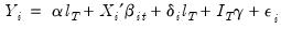
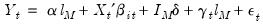
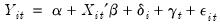
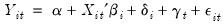
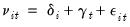
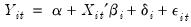
The basic class of models that can be estimated using a pool object may be written as:
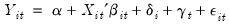 | (53.2) |
where

is the dependent variable, and

is a

‑vector of regressors, and

are the error terms for
cross-sectional units observed for dated periods
. The

parameter represents the overall constant in the model, while the

and

represent cross-section or period specific effects (random or fixed). Identification obviously requires that the

coefficients have restrictions placed upon them. They may be divided into sets of common (across cross-section and periods), cross-section specific, and period specific regressor parameters.
While most of our discussion will be in terms of a balanced sample, EViews does not require that your data be balanced; missing values may be used to represent observations that are not available for analysis in a given period. We will detail the unbalanced case only where deemed necessary.
We may view these data as a set of cross-section specific regressions so that we have

cross-sectional equations each with

observations stacked on top of one another:
 | (53.3) |
for

, where

is a

-element unit vector,

is the

-element identity matrix, and

is a vector containing all of the period effects,
.
Analogously, we may write the specification as a set of

period specific equations, each with

observations stacked on top of one another.
 | (53.4) |
for

, where

is a

-element unit vector,

is the

-element identity matrix, and

is a vector containing all of the cross-section effects,
.
For purposes of discussion we will employ the stacked representation of these equations. First, for the specification organized as a set of cross-section equations, we have:
 | (53.5) |
where the matrices

and

are set up to impose any restrictions on the data and parameters between cross-sectional units and periods, and where the general form of the unconditional error covariance matrix is given by:
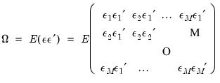 | (53.6) |
If instead we treat the specification as a set of period specific equations, the stacked (by period) representation is given by,
 | (53.7) |
with error covariance,
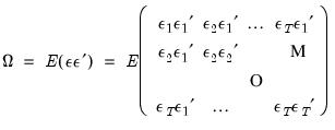 | (53.8) |
The remainder of this section describes briefly the various components that you may employ in an EViews pool specification.
Cross-section and Period Specific Regressors
The basic EViews pool specification in
Equation (53.2) allows for

slope coefficients that are common to all individuals and periods, as well as coefficients that are either cross-section or period specific. Before turning to the general specification, we consider three extreme cases.
First, if all of the

are common across cross-sections and periods, we may simplify the expression for
Equation (53.2) to:
 | (53.9) |
There are a total of

coefficients in

, each corresponding to an element of

.
Alternately, if all of the

coefficients are cross-section specific, we have:
 | (53.10) |
Note that there are

in each

for a total of

slope coefficients.
Lastly, if all of the

coefficients are period specific, the specification may be written as:
 | (53.11) |
for a total of

slope coefficients.
More generally, splitting

into the three groups (common regressors

, cross-section specific regressors

, and period specific regressors

), we have:
 | (53.12) |
If there are

common regressors,

cross-section specific regressors, and

period specific regressors, there are a total of
regressors in

.
EViews estimates these models by internally creating interaction variables,

for each regressor in the cross-section regressor list and

for each regressor in the period-specific list, and using them in the regression. Note that estimating models with cross-section or period specific coefficients may lead to the generation of a large number of implicit interaction variables, and may be computationally intensive, or lead to singularities in estimation.
AR Specifications
EViews provides convenient tools for estimating pool specifications that include AR terms. Consider a restricted version of
Equation (53.2) that does not admit period specific regressors or effects,
 | (53.13) |
where the cross-section effect

is either not present, or is specified as a fixed effect. We then allow the residuals to follow a general AR process:
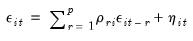 | (53.14) |
for all

, where the innovations

are independent and identically distributed, assuming further that there is no unit root. Note that we allow the autocorrelation coefficients

to be cross-section, but not period specific.
If, for example, we assume that

follows an AR(1) process with cross-section specific AR coefficients, EViews will estimate the transformed equation:
 | (53.15) |
using iterative techniques to estimate (

) for all

. See
“Specifying AR Terms” for additional discussion.
We emphasize that EViews does place are restrictions on the specifications that admit AR errors. AR terms may not be estimated in specifications with period specific regressors or effects. Lastly, AR terms are not allowed in selected GLS specifications (random effects, period specific heteroskedasticity and period SUR). In those GLS specifications where AR terms are allowed, the error covariance assumption is for the innovations not the autoregressive error.
Fixed and Random Effects
The presence of cross-section and period specific effects terms

and

may be handled using fixed or random effects methods.
You may, with some restrictions, specify models containing effects in one or both dimension, for example, a fixed effect in the cross-section dimension, a random effect in the period dimension, or a fixed effect in the cross-section and a random effect in the period dimension. Note, in particular, however, that two-way random effects may only be estimated if the data are balanced so that every cross-section has the same set of observations.
Fixed Effects
The fixed effects portions of specifications are handled using orthogonal projections. In the simple one-way fixed effect specifications and the balanced two-way fixed specification, these projections involve the familiar approach of removing cross-section or period specific means from the dependent variable and exogenous regressors, and then performing the specified regression using the demeaned data (see, for example Baltagi, 2005). More generally, we apply the results from Davis (2002) for estimating multi-way error components models with unbalanced data.
Note that if instrumental variables estimation is specified with fixed effects, EViews will automatically add to the instrument list, the constants implied by the fixed effects so that the orthogonal projection is also applied to the instrument list.
Random Effects
The random effects specifications assumes that the corresponding effects

and

are realizations of independent random variables with mean zero and finite variance. Most importantly, the random effects specification assumes that the effect is uncorrelated with the idiosyncratic residual

.
EViews handles the random effects models using feasible GLS techniques. The first step, estimation of the covariance matrix for the composite error formed by the effects and the residual (
e.g.,
in the two-way random effects specification), uses one of the quadratic unbiased estimators (QUE) from Swamy-Arora, Wallace-Hussain, or Wansbeek-Kapteyn. Briefly, the three QUE methods use the expected values from quadratic forms in one or more sets of first-stage estimated residuals to compute moment estimates of the component variances

. The methods differ only in the specifications estimated in evaluating the residuals, and the resulting forms of the moment equations and estimators.
The Swamy-Arora estimator of the component variances, cited most often in textbooks, uses residuals from the within (fixed effect) and between (means) regressions. In contrast, the Wansbeek and Kapteyn estimator uses only residuals from the fixed effect (within) estimator, while the Wallace-Hussain estimator uses only OLS residuals. In general, the three should provide similar answers, especially in large samples. The Swamy-Arora estimator requires the calculation of an additional model, but has slightly simpler expressions for the component variance estimates. The remaining two may prove easier to estimate in some settings.
Additional details on random effects models are provided in Baltagi (2005), Baltagi and Chang (1994), Wansbeek and Kapteyn (1989). Note that your component estimates may differ slightly from those obtained from other sources since EViews always uses the more complicated unbiased estimators involving traces of matrices that depend on the data (see Baltagi (2005) for discussion, especially “Note 3” on p. 28).
Once the component variances have been estimated, we form an estimator of the composite residual covariance, and then GLS transform the dependent and regressor data.
If instrumental variables estimation is specified with random effects, EViews will GLS transform both the data and the instruments prior to estimation. This approach to random effects estimation has been termed generalized two-stage least squares (G2SLS). See Baltagi (2005, p. 113-116) and
“Random Effects and GLS” for additional discussion.
Generalized Least Squares
You may estimate GLS specifications that account for various patterns of correlation between the residuals. There are four basic variance structures that you may specify: cross-section specific heteroskedasticity, period specific heteroskedasticity, contemporaneous covariances, and between period covariances.
Note that all of the GLS specifications described below may be estimated in one-step form, where we estimate coefficients, compute a GLS weighting transformation, and then reestimate on the weighted data, or in iterative form, where to repeat this process until the coefficients and weights converge.
Cross-section Heteroskedasticity
Cross-section heteroskedasticity allows for a different residual variance for each cross section. Residuals between different cross-sections and different periods are assumed to be 0. Thus, we assume that:
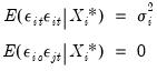 | (53.16) |
for all

,

,

and

with

and

, where

contains

and, if estimated by fixed effects, the relevant cross-section or period effects (

).
Using the cross-section specific residual vectors, we may rewrite the main assumption as:
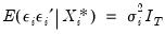 | (53.17) |
GLS for this specification is straightforward. First, we perform preliminary estimation to obtain cross-section specific residual vectors, then we use these residuals to form estimates of the cross-specific variances. The estimates of the variances are then used in a weighted least squares procedure to form the feasible GLS estimates.
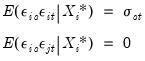
Period Heteroskedasticity
Exactly analogous to the cross-section case, period specific heteroskedasticity allows for a different residual variance for each period. Residuals between different cross-sections and different periods are still assumed to be 0 so that:
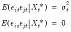 | (53.18) |
for all

,

,

and

with

, where

contains

and, if estimated by fixed effects, the relevant cross-section or period effects (

).
Using the period specific residual vectors, we may rewrite the first assumption as:
 | (53.19) |
We perform preliminary estimation to obtain period specific residual vectors, then we use these residuals to form estimates of the period variances, reweight the data, and then form the feasible GLS estimates.
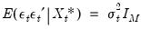
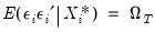
Contemporaneous Covariances (Cross-section SUR)
This class of covariance structures allows for conditional correlation between the contemporaneous residuals for cross-section

and

, but restricts residuals in different periods to be uncorrelated. Specifically, we assume that:
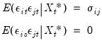 | (53.20) |
for all

,

,

and

with

. The errors may be thought of as cross-sectionally correlated. Alternately, this error structure is sometimes referred to as clustered by period since observations for a given period are correlated (form a cluster). Note that in this specification the contemporaneous covariances do not vary over

.
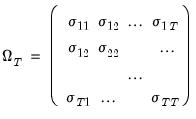
Using the period specific residual vectors, we may rewrite this assumption as,
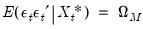 | (53.21) |
for all

, where,
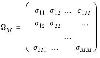 | (53.22) |
We term this a Cross-section SUR specification since it involves covariances across cross-sections as in a seemingly unrelated regressions type framework (where each equation corresponds to a cross-section).
Cross-section SUR generalized least squares on this specification (sometimes referred to as the Parks estimator) is simply the feasible GLS estimator for systems where the residuals are both cross-sectionally heteroskedastic and contemporaneously correlated. We employ residuals from first stage estimates to form an estimate of

. In the second stage, we perform feasible GLS.
Bear in mind that there are potential pitfalls associated with the SUR/Parks estimation (see Beck and Katz (1995)). For one, EViews may be unable to compute estimates for this model when you the dimension of the relevant covariance matrix is large and there are a small number of observations available from which to obtain covariance estimates. For example, if we have a cross-section SUR specification with large numbers of cross-sections and a small number of time periods, it is quite likely that the estimated residual correlation matrix will be nonsingular so that feasible GLS is not possible.
It is worth noting that an attractive alternative to the SUR methodology estimates the model without a GLS correction, then corrects the coefficient estimate covariances to account for the contemporaneous correlation. See
“Robust Coefficient Covariances”.
Note also that if cross-section SUR is combined with instrumental variables estimation, EViews will employ a Generalized Instrumental Variables estimator in which both the data and the instruments are transformed using the estimated covariances. See Wooldridge (2002) for discussion and comparison with the three-stage least squares approach.
Serial Correlation (Period SUR)
This class of covariance structures allows for arbitrary heteroskedasticity and serial correlation between the residuals for a given cross-section, but restricts residuals in different cross-sections to be uncorrelated. This error structure is sometimes referred to as clustered by cross-section since observations in a given cross-section are correlated (form a cluster).
Accordingly, we assume that:
 | (53.23) |
for all

,

,

and

with

. Note that in this specification the heteroskedasticity and serial correlation does not vary across cross-sections

.
Using the cross-section specific residual vectors, we may rewrite this assumption as,
 | (53.24) |
for all

, where,
 | (53.25) |
We term this a
Period SUR specification since it involves covariances across periods within a given cross-section, as in a seemingly unrelated regressions framework with period specific equations. In estimating a specification with Period SUR, we employ residuals obtained from first stage estimates to form an estimate of

. In the second stage, we perform feasible GLS.
See
“Contemporaneous Covariances (Cross-section SUR)” for related discussion of errors clustered-by-period.
Instrumental Variables
All of the pool specifications may be estimated using instrumental variables techniques. In general, the computation of the instrumental variables estimator is a straightforward extension of the standard OLS estimator. For example, in the simplest model, the OLS estimator may be written as:
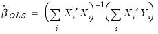 | (53.26) |
while the corresponding IV estimator is given by:
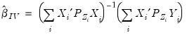 | (53.27) |
where

is the orthogonal projection matrix onto the

.
There are, however, additional complexities introduced by instruments that require some discussion.
Cross-section and Period Specific Instruments
As with the regressors, we may divide the instruments into three groups (common instruments

, cross-section specific instruments

, and period specific instruments

).
You should make certain that any exogenous variables in the regressor groups are included in the corresponding instrument groups, and be aware that each entry in the latter two groups generates multiple instruments.
Fixed Effects
If instrumental variables estimation is specified with fixed effects, EViews will automatically add to the instrument list any constants implied by the fixed effects so that the orthogonal projection is also applied to the instrument list. Thus, if

is the fixed effects transformation operator, we have:
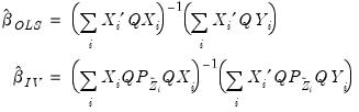 | (53.28) |
where

.
Random Effects and GLS
Similarly, for random effects and other GLS estimators, EViews applies the weighting to the instruments as well as the dependent variable and regressors in the model. For example, with data estimated using cross-sectional GLS, we have:
 | (53.29) |
where
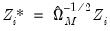
.
In the context of random effects specifications, this approach to IV estimation is termed generalized two-stage least squares (G2SLS) method (see Baltagi (2005, p. 113-116) for references and discussion). Note that in implementing the various random effects methods (Swamy-Arora, Wallace-Hussain, Wansbeek-Kapteyn), we have extended the existing results to derive the unbiased variance components estimators in the case of instrumental variables estimation.
More generally, the approach may simply be viewed as a special case of the Generalized Instrumental Variables (GIV) approach in which data and the instruments are both transformed using the estimated covariances. You should be aware that this has approach has the effect of altering the implied orthogonality conditions. See Wooldridge (2002) for discussion and comparison with a three-stage least squares approach in which the instruments are not transformed. See
“GMM Details” for an alternative approach.
AR Specifications
EViews estimates AR specifications by transforming the data to a nonlinear least squares specification, and jointly estimating the original and the AR coefficients.
This transformation approach raises questions as to what instruments to use in estimation. By default, EViews adds instruments corresponding to the lagged endogenous and lagged exogenous variables introduced into the specification by the transformation.
For example, in an AR(1) specification, we have the original specification,
 | (53.30) |
and the transformed equation,
 | (53.31) |
where

and

are introduced by the transformation. EViews will, by default, add these to the previously specified list of instruments

.
You may, however, instruct EViews not to add these additional instruments. Note, however, that the order condition for the transformed model is different than the order condition for the untransformed specification since we have introduced additional coefficients corresponding to the AR coefficients. If you elect not to add the additional instruments automatically, you should make certain that you have enough instruments to account for the additional terms.
Robust Coefficient Covariances
In this section, we describe the basic features of the various robust estimators, for clarity focusing on the simple cases where we compute robust covariances for models estimated by standard OLS without cross-section or period effects. The extensions to models estimated using instrumental variables, fixed or random effects, and GLS weighted least squares are straightforward.
White Robust Covariances
The White cross-section (period cluster) method assumes that the errors are contemporaneously (cross-sectionally) correlated. The method treats the pool regression as a multivariate regression (with an equation for each cross-section), and computes robust standard errors for the system of equations. This estimator is robust to cross-equation (contemporaneous) correlation and heteroskedasticity. See Wooldridge (2002, p. 148-153) and Arellano (1987).
Alternatively, the White period (cross-section cluster) method assumes that the errors for a cross-section are heteroskedastic and serially correlated. The estimator is designed to accommodate arbitrary heteroskedasticity and within cross-section serial correlation.
The White two-way cluster method allows for both cross-section and period clustering.
In contrast, the White (diagonal) method is robust to observation specific heteroskedasticity in the disturbances, but not to correlation between residuals for different observations.
Each of the coefficient covariance methods is described in greater detail in
“Cluster-Robust Covariances”.
PCSE Robust Covariances
The remaining methods are variants of the first two White statistics in which residuals are replaced by moment estimators for the unconditional variances. These methods, which are variants of the so-called
Panel Corrected Standard Error (PCSE) methodology (Beck and Katz, 1995), are robust to unrestricted unconditional variance matrices

and

, but place additional restrictions on the conditional variance matrices.
A sufficient (though not necessary) condition for use of PCSE is that the conditional and unconditional variances are the same. (Note also that as with the SUR estimators above, we require that

and
 not
not vary with

and

, respectively.)
For example, the
Cross-section SUR (PCSE) method handles cross-section correlation (period clustering) by replacing the outer product of the cross-section residuals in the White cross-section (period clustered) computation with an estimate of the (contemporaneous) cross-section residual covariance matrix

:
Analogously, the
Period SUR (PCSE) handles between period correlation (cross-section clustering) by replacing the outer product of the period residuals in the White period (cross-section clustered) computation with an estimate of the period covariance

:
The two diagonal forms of these estimators, Cross-section weights (PCSE), and Period weights (PCSE), use only the diagonal elements of the relevant

and

. These covariance estimators are robust to heteroskedasticity across cross-sections or periods, respectively, but not to general correlation of residuals.
The non degree-of-freedom corrected versions of these estimators remove the leading term involving the number of observations and number of coefficients.