Background
We present here a brief discussion of quantile regression. As always, the discussion is necessarily brief and omits considerable detail. For a book-length treatment of quantile regression see Koenker (2005).
The Model
Suppose that we have a random variable

with probability distribution function
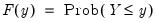 | (40.2) |
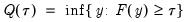
so that for

, the

-th quantile of

may be defined as the smallest

satisfying

:
 | (40.3) |
Given a set of

observations on

, the traditional empirical distribution function is given by:
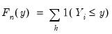 | (40.4) |
where

is an indicator function that takes the value 1 if the argument

is true and 0 otherwise. The associated empirical quantile is given by,
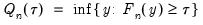 | (40.5) |
or equivalently, in the form of a simple optimization problem:
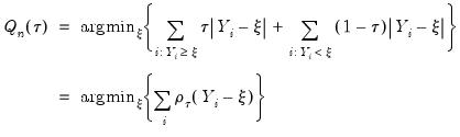 | (40.6) |
where

is the so-called
check function which weights positive and negative values asymmetrically.
Quantile regression extends this simple formulation to allow for regressors

. We assume a linear specification for the conditional quantile of the response variable

given values for the

-vector of explanatory variables

:
 | (40.7) |
where

is the vector of coefficients associated with the

-th quantile.
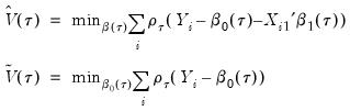
Then the analog to the unconditional quantile minimization above is the conditional quantile regression estimator:
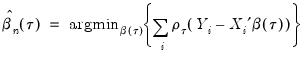 | (40.8) |
Estimation
The quantile regression estimator can be obtained as the solution to a linear programming problem. Several algorithms for obtaining a solution to this problem have been proposed in the literature. EViews uses a modified version of the Koenker and D’Orey (1987) version of the Barrodale and Roberts (1973) simplex algorithm.
The Barrodale and Roberts (BR) algorithm has received more than its fair share of criticism for being computationally inefficient, with dire theoretical results for worst-case scenarios in problems involving large numbers of observations. Simulations showing poor relative performance of the BR algorithm as compared with alternatives such as interior point methods appear to bear this out, with estimation times that are roughly quadratic in the number of observations (Koenker and Hallock, 2001; Portnoy and Koenker, 1997).
Our experience with our optimized version of the BR algorithm is that its performance is certainly better than commonly portrayed. Using various subsets of the low-birthweight data described in Koenker and Hallock (2001), we find that while certainly not as fast as Cholesky-based linear regression (and possibly not as fast as interior point methods), the estimation times for the modified BR algorithm are quite reasonable.
For example, estimating a 16 explanatory variable model for the median using the first 20,000 observations of the data set takes a bit more than 1.2 seconds on a 3.2GHz Pentium 4, with 1.0Gb of RAM; this time includes both estimation and computation of a kernel based estimator of the coefficient covariance matrix. The same specification using the full sample of 198,377 observations takes under 7.5 seconds.
Overall, our experience is that estimation times for the modified BR algorithm are roughly linear in the number of observations through a broad range of sample sizes. While our results are not definitive, we see no real impediment to using this algorithm for virtually all practical problems.
Asymptotic Distributions
Under mild regularity conditions, quantile regression coefficients may be shown to be asymptotically normally distributed (Koenker, 2005) with different forms of the asymptotic covariance matrix depending on the model assumptions.
Computation of the coefficient covariance matrices occupies an important place in quantile regression analysis. In large part, this importance stems from the fact that the covariance matrix of the estimates depends on one or more nuisance quantities which must be estimated. Accordingly, a large literature has developed to consider the relative merits of various approaches to estimating the asymptotic variances (see Koenker (2005), for an overview).
We may divide the estimators into three distinct classes: (1) direct methods for estimating the covariance matrix in i.i.d. settings; (2) direct methods for estimating the covariance matrix for independent but not-identical distribution; (3) bootstrap resampling methods for both i.i.d. and i.n.i.d. settings.
Independent and Identical
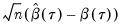
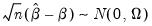
Koenker and Bassett (1978) derive asymptotic normality results for the quantile regression estimator in the i.i.d. setting, showing that under mild regularity conditions,
 | (40.9) |
where:
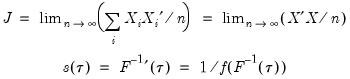 | (40.10) |
and

, which is termed the
sparsity function or the
quantile density function, may be interpreted either as the derivative of the quantile function or the inverse of the density function evaluated at the

-th quantile (see, for example, Welsh, 1988). Note that the
i.i.d. error assumption implies that

does not depend on

so that the quantile functions depend on

only in location, hence all conditional quantile planes are parallel.
Given the value of the sparsity at a given quantile, direct estimation of the coefficient covariance matrix is straightforward. In fact, the expression for the asymptotic covariance in
Equation (40.9) is analogous to the ordinary least squares covariance in the
i.i.d. setting, with

standing in for the error variance in the usual formula.
Sparsity Estimation
We have seen the importance of the sparsity function in the formula for the asymptotic covariance matrix of the quantile regression estimates for
i.i.d. data. Unfortunately, the sparsity is a function of the unknown distribution

, and therefore is a nuisance quantity which must be estimated.
EViews provides three methods for estimating the scalar sparsity

: two Siddiqui (1960) difference quotient methods (Koenker, 1994; Bassett and Koenker (1982) and one kernel density estimator (Powell, 1986; Jones, 1992; Buchinsky 1995).
Siddiqui Difference Quotient
The first two methods are variants of a procedure originally proposed by Siddiqui (1960; see Koenker, 1994), where we compute a simple difference quotient of the empirical quantile function:
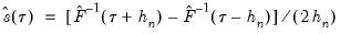 | (40.11) |
for some bandwidth

tending to zero as the sample size

.

is in essence computed using a simply two-sided numeric derivative of the quantile function. To make this procedure operational we need to determine: (1) how to obtain estimates of the empirical quantile function

at the two evaluation points, and (2) what bandwidth to employ.
The first approach to evaluating the quantile functions, which EViews terms is due to Bassett and Koenker (1982). The approach involves estimating two additional quantile regression models for

and

, and using the estimated coefficients to compute fitted quantiles. Substituting the fitted quantiles into the numeric derivative expression yields:
 | (40.12) |
for an arbitrary

. While the
i.i.d. assumption implies that

may be set to any value, Bassett and Koenker propose using the mean value of

, noting that the mean possesses two very desirable properties: the precision of the estimate is maximized at that point, and the empirical quantile function is monotone in

when evaluated at

, so that

will always yield a positive value for suitable

.
A second, less computationally intensive approach to evaluating the quantile functions computes the

and

empirical quantiles of the residuals from the original quantile regression equation, as in Koenker (1994). Following Koencker, we compute quantiles for the residuals excluding the

residuals that are set to zero in estimation, and interpolating values to get a piecewise linear version of the quantile. EViews refers to this method as .
Both Siddiqui methods require specification of a bandwidth

. EViews offers the Bofinger (1975), Hall-Sheather (1988), and Chamberlain (1994) bandwidth methods (along with the ability to specify an arbitrary bandwidth).
The Bofinger bandwidth, which is given by:
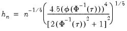 | (40.13) |
(approximately) minimizes the mean square error (MSE) of the sparsity estimates.
Hall-Sheather proposed an alternative bandwidth that is designed specifically for testing. The Hall-Sheather bandwidth is given by:
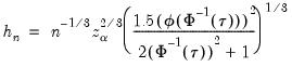 | (40.14) |
where
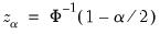
, for

the parameter controlling the size of the desired

confidence intervals.
A similar testing motivation underlies the Chamberlain bandwidth:
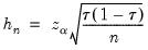 | (40.15) |
which is derived using the exact and normal asymptotic confidence intervals for the order statistics (Buchinsky, 1995).
Kernel Density
Kernel density estimators of the sparsity offer an important alternative to the Siddiqui approach. Most of the attention has focused on kernel methods for estimating the derivative

directly (Falk, 1988; Welsh, 1988), but one may also estimate

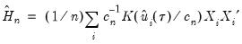
using the inverse of a kernel density function estimator (Powell, 1986; Jones, 1992; Buchinsky 1995). In the present context, we may compute:
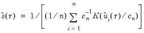 | (40.16) |
where

are the residuals from the quantile regression fit. EViews supports the latter density function approach, which is termed the method, since it is closely related to the more commonly employed Powell (1984, 1989) kernel estimator for the non-
i.i.d. case described below.
Kernel estimation of the density function requires specification of a bandwidth

. We follow Koenker (2005, p. 81) in choosing:
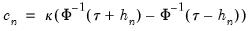 | (40.17) |
where
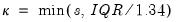
is the Silverman (1986) robust estimate of scale (where

the sample standard deviation and

the interquartile range) and

is the Siddiqui bandwidth.
Independent, Non-Identical
We may relax the assumption that the quantile density function does not depend on

. The asymptotic distribution of
in the
i.n.i.d. setting takes the Huber sandwich form (see, among others, Hendricks and Koenker, 1992):
 | (40.18) |
where

is as defined earlier,
 | (40.19) |
and:
 | (40.20) |

is the conditional density function of the response, evaluated at the

-th conditional quantile for individual

. Note that if the conditional density does not depend on the observation, the Huber sandwich form of the variance in
Equation (40.18) reduces to the simple scalar sparsity form given in
Equation (40.9).
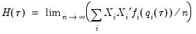
Computation of a sample analogue to

is straightforward so we focus on estimation of

. EViews offers a choice of two methods for estimating

: a Siddiqui-type difference method proposed by Hendricks and Koenker (1992), and a Powell (1984, 1989) kernel method based on residuals of the estimated model. EViews labels the first method , and the latter method :
The Siddiqui-type method proposed by Hendricks and Koenker (1991) is a straightforward generalization of the scalar Siddiqui method (see
“Siddiqui Difference Quotient”). As before, two additional quantile regression models are estimated for

and

, and the estimated coefficients may be used to compute the Siddiqui difference quotient:
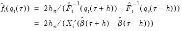 | (40.21) |
Note that in the absence of identically distributed data, the quantile density function

must be evaluated for each individual. One minor complication is that
Equation (40.21) is not guaranteed to be positive except at

. Accordingly, Hendricks and Koenker modify the expression slightly to use only positive values:
 | (40.22) |
where

is a small positive number included to prevent division by zero.
The estimated quantile densities

are then used to form an estimator

of

:
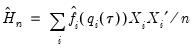 | (40.23) |
The Powell (1984, 1989) kernel approach replaces the Siddiqui difference with a kernel density estimator using the residuals of the original fitted model:
 | (40.24) |
where

is a kernel function that integrates to 1, and

is a kernel bandwidth. EViews uses the Koenker (2005) kernel bandwidth as described in
“Kernel Density” above.
Bootstrapping
The direct methods of estimating the asymptotic covariance matrices of the estimates require the estimation of the sparsity nuisance parameter, either at a single point, or conditionally for each observation. One method of avoiding this cumbersome estimation is to employ bootstrapping techniques for the estimation of the covariance matrix.
EViews supports four different bootstrap methods: the residual bootstrap (), the design, or XY-pair, bootstrap (), and two variants of the Markov Chain Marginal Bootstrap ( and ).
The following discussion provides a brief overview of the various bootstrap methods. For additional detail, see Buchinsky (1995, He and Hu (2002) and Kocherginsky, He, and Mu (2005).
Residual Bootstrap
The
residual bootstrap, is constructed by resampling (with replacement) separately from the residuals

and from the

.
Let

be an

-vector of resampled residuals, and let

be a

matrix of independently resampled

. (Note that

need not be equal to the original sample size

.) We form the dependent variable using the resampled residuals, resampled data, and estimated coefficients,
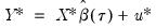
, and then construct a bootstrap estimate of

using

and

.
This procedure is repeated for

bootstrap replications, and the estimator of the asymptotic covariance matrix is formed from:
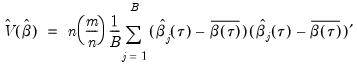 | (40.25) |
where

is the mean of the bootstrap elements. The bootstrap covariance matrix

is simply a (scaled) estimate of the sample variance of the bootstrap estimates of

.
Note that the validity of using separate draws from

and

requires independence of the

and the

.
XY-pair (Design) Bootstrap
The
XY-pair bootstrap is the most natural form of bootstrap resampling, and is valid in settings where

and

are not independent. For the XY-pair bootstrap, we simply form

randomly drawn (with replacement) subsamples of size

from the original data, then compute estimates of

using the

for each subsample. The asymptotic covariance matrix is then estimated from sample variance of the bootstrap results using
Equation (40.25).
Markov Chain Marginal Bootstrap
The primary disadvantage to the residual and design bootstrapping methods is that they are computationally intensive, requiring estimation of a relatively difficult

-dimensional linear programming problem for each bootstrap replication.
He and Hu (2002) proposed a new method for constructing bootstrap replications that reduces each

-dimensional bootstrap optimization to a sequence of

easily solved one-dimensional problems. The sequence of one-dimensional solutions forms a Markov chain whose sample variance, computed using
Equation (40.25), consistently approximates the true covariance for large

and

.
One problem with the MCMB is that high autocorrelations in the MCMB sequence for specific coefficients will result in a poor estimates for the asymptotic covariance for given chain length

, and may result in non-convergence of the covariance estimates for any chain of practical length.
Kocherginsky, He, and Mu (KHM, 2005) propose a modification to MCMB, which alleviates autocorrelation problems by transforming the parameter space prior to performing the MCMB algorithm, and then transforming the result back to the original space. Note that the resulting MCMB-A algorithm requires the i.i.d. assumption, though the authors suggest that the method is robust against heteroskedasticity.
Practical recommendations for the MCMB-A are provided in KHM. Summarizing, they recommend that the methods be applied to problems where
with

between 100 and 200 for relatively small problems (
). For moderately large problems with

between 10,000 and 2,000,000, they recommend

between 50 and 200 depending on one’s level of patience.
Model Evaluation and Testing
Evaluation of the quality of a quantile regression model may be conducted using goodness-of-fit criteria, as well as formal testing using quasi-likelihood ratio and Wald tests.
Goodness-of-Fit
Koenker and Machado (1999) define a goodness-of-fit statistic for quantile regression that is analogous to the

from conventional regression analysis. We begin by recalling our linear quantile specification,
and assume that we may partition the data and coefficient vector as
and
, so that
 | (40.26) |
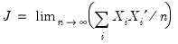
We may then define:
 | (40.27) |
the minimized unrestricted and intercept-only objective functions. The Koenker and Machado goodness-of-fit criterion is given by:
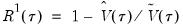 | (40.28) |
This statistic is an obvious analogue of the conventional

.

lies between 0 and 1, and measures the relative success of the model in fitting the data for the

-th quantile.
Quasi-Likelihood Ratio Tests
Koenker and Machado (1999) describe quasi-likelihood ratio tests based on the change in the optimized value of the objective function after relaxation of the restrictions imposed by the null hypothesis. They offer two test statistics which they term
quantile-
tests, though as Koenker (2005) points out, they may also be thought of as quasi-likelihood ratio tests.
We define the test statistics:
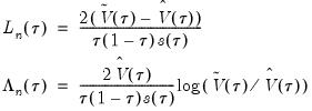 | (40.29) |
which are both asymptotically

where

is the number of restrictions imposed by the null hypothesis.
You should note the presence of the sparsity term

in the denominator of both expressions. Any of the sparsity estimators outlined in
“Sparsity Estimation” may be employed for either the null or alternative specifications; EViews uses the sparsity estimated under the alternative. The presence of

should be a tipoff that these test statistics require that the quantile density function does not depend on

, as in the pure location-shift model.
Note that EViews will always compute an estimate of the scalar sparsity, even when you specify a Huber sandwich covariance method. This value of the sparsity will be used to compute QLR test statistics which may be less robust than the corresponding Wald counterparts.
Coefficient Tests
Given estimates of the asymptotic covariance matrix for the quantile regression estimates, you may construct Wald-type tests of hypotheses and construct coefficient confidence ellipses as in
“Coefficient Diagnostics”.
Quantile Process Testing
The focus of our analysis thus far has been on the quantile regression model for a single quantile,

. In a number of cases, we may instead be interested in forming joint hypotheses using coefficients for more than one quantile. We may, for example, be interested in evaluating whether the location-shift model is appropriate by testing for equality of slopes across quantile values. Consideration of more than one quantile regression at the same time comes under the general category of
quantile process analysis.
While the EViews equation object is set up to consider only one quantile at a time, specialized tools allow you to perform the most commonly performed quantile process analyses.
Before proceeding to the hypothesis tests of interest, we must first outline the required distributional theory. Define the process coefficient vector:
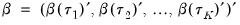 | (40.30) |
Then
 | (40.31) |
where

has blocks of the form:
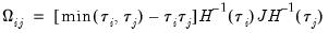 | (40.32) |
In the
i.i.d. setting,

simplifies to,
 | (40.33) |
where

has representative element:
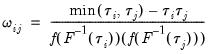 | (40.34) |
Estimation of

may be performed directly using
(40.32),
(40.33) and
(40.34), or using one of the bootstrap variants.
Slope Equality Testing
Koenker and Bassett (1982a) propose testing for slope equality across quantiles as a robust test of heteroskedasticity. The null hypothesis is given by:
 | (40.35) |
which imposes
restrictions on the coefficients. We may form the corresponding Wald statistic, which is distributed as a

.
Symmetry Testing
Newey and Powell (1987) construct a test of the less restrictive hypothesis of symmetry, for asymmetric least squares estimators, but the approach may easily be applied to the quantile regression case.
The premise of the Newey and Powell test is that if the distribution of

given

is symmetric, then:
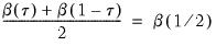 | (40.36) |
We may evaluate this restriction using Wald tests on the quantile process. Suppose that there are an odd number,

, of sets of estimated coefficients ordered by

. The middle value

is assumed to be equal to 0.5, and the remaining

are symmetric around 0.5, with
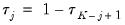
, for

. Then the Newey and Powell test null is the joint hypothesis that:
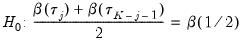 | (40.37) |
for
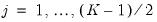
.
The Wald test formed for this null is zero under the null hypothesis of symmetry. The null has

restrictions, so the Wald statistic is distributed as a

. Newey and Powell point out that if it is known
a priori that the errors are
i.i.d., but possibly asymmetric, one can restrict the null to only examine the restriction for the intercept. This restricted null imposes only

restrictions on the process coefficients.