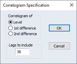
 at lag
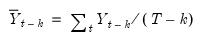
  is estimated by:
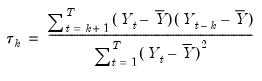 | (11.24) |
 is the sample mean of
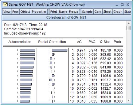
  . This is the correlation coefficient for values of the series
  periods apart. If
  is nonzero, it means that the series is first order serially correlated. If
  dies off more or less geometrically with increasing lag
  , it is a sign that the series obeys a low-order autoregressive (AR) process. If
  drops to zero after a small number of lags, it is a sign that the series obeys a low-order moving-average (MA) process. See
“Background” for a more complete description of AR and MA processes.
drops to zero after a small number of lags, it is a sign that the series obeys a low-order moving-average (MA) process. See
“Background” for a more complete description of AR and MA processes.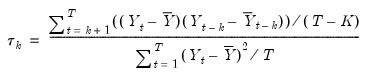 | (11.25) |
 . The difference arises since, for computational simplicity, EViews employs the same overall sample mean
  as the mean of both
  and
and  . While both formulations are consistent estimators, the EViews formulation biases the result toward zero in finite samples.
 . If the autocorrelation is within these bounds, it is not significantly different from zero at (approximately) the 5% significance level.
  is the regression coefficient on
  when
when  is regressed on a constant,
 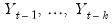 . This is a partial correlation since it measures the correlation of
  values that are
  periods apart after removing the correlation from the intervening lags. If the pattern of autocorrelation is one that can be captured by an autoregression of order less than
  , then the partial autocorrelation at lag
  will be close to zero.
 , AR(
, AR( ), cuts off at lag
  , while the PAC of a pure moving average (MA) process asymptotes gradually to zero.
  recursively by
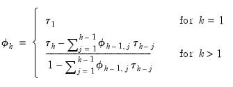 | (11.26) |
 is the estimated autocorrelation at lag
  and where,
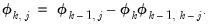 | (11.27) |
 , simply run the regression:
 | (11.28) |
 is a residual. The dotted lines in the plots of the partial autocorrelations are the approximate two standard error bounds computed as
  . If the partial autocorrelation is within these bounds, it is not significantly different from zero at (approximately) the 5% significance level.
 is a test statistic for the null hypothesis that there is no autocorrelation up to order
  and is computed as:
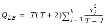 | (11.29) |
 is the j-th autocorrelation and
  is the number of observations. If the series is not based upon the results of ARIMA estimation, then under the null hypothesis, Q is asymptotically distributed as a
  with degrees of freedom equal to the number of autocorrelations. If the series represents the residuals from ARIMA estimation, the appropriate degrees of freedom should be adjusted to represent the number of autocorrelations less the number of AR and MA terms previously estimated. Note also that some care should be taken in interpreting the results of a Ljung-Box test applied to the residuals from an ARMAX specification (see Dezhbaksh, 1990, for simulation evidence on the finite sample performance of the test in this setting).