Frequency (Band-Pass) Filter
EViews computes several forms of band-pass (frequency) filters. These filters are used to isolate the cyclical component of a time series by specifying a range for its duration. Roughly speaking, the band-pass filter is a linear filter that takes a two-sided weighted moving average of the data where cycles in a “band”, given by a specified lower and upper bound, are “passed” through, or extracted, and the remaining cycles are “filtered” out.
To employ a band-pass filter, the user must first choose the range of durations (
periodicities) to pass through. The range is described by a pair of numbers

, specified in units of the workfile frequency. Suppose, for example, that you believe that the business cycle lasts somewhere from 1.5 to 8 years so that you wish to extract the cycles in this range. If you are working with quarterly data, this range corresponds to a low duration of 6, and an upper duration of 32 quarters. Thus, you should set

and

.
In some contexts, it will be useful to think in terms of frequencies which describe the number of cycles in a given period (obviously, periodicities and frequencies are inversely related). By convention, we will say that periodicities in the range

correspond to frequencies in the range
.
Note that since saying that we have a cycle with a period of 1 is meaningless, we require that

. Setting

to the lower-bound value of 2 yields a
high-pass filter in which all frequencies above

are passed through.
The various band-pass filters differ in the way that they compute the moving average:
• The fixed length symmetric filters employ a fixed lead/lag length. Here, the user must specify the fixed number of lead and lag terms to be used when computing the weighted moving average. The symmetric filters are time-invariant since the moving average weights depend only on the specified frequency band, and do not use the data. EViews computes two variants of this filter, the first due to Baxter-King (1999) (BK), and the second to Christiano-Fitzgerald (2003) (CF). The two forms differ in the choice of objective function used to select the moving average weights.
• Full sample asymmetric – this is the most general filter, where the weights on the leads and lags are allowed to differ. The asymmetric filter is time-varying with the weights both depending on the data and changing for each observation. EViews computes the Christiano-Fitzgerald (CF) form of this filter.
In choosing between the two methods, bear in mind that the fixed length filters require that we use same number of lead and lag terms for every weighted moving average. Thus, a filtered series computed using

leads and lags observations will lose

observations from both the beginning and end of the original sample. In contrast, the asymmetric filtered series do not have this requirement and can be computed to the ends of the original sample.
Computing a Band-Pass Filter in EViews
The band-pass filter is available as a series Proc in EViews. To display the band-pass filter dialog, select from the main series menu.
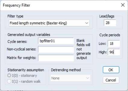
The first thing you will do is to select a filter type. There are three types: , , or . By default, the EViews will compute the Baxter-King fixed length symmetric filter.
For the Baxter-King filter, there are only a few options that require your attention. First, you must select a frequency length (lead/lags) for the moving average, and the low and high values for the cycle period

to be filtered. By default, these fields will be filled in with reasonable default values that are based on the type of your workfile.
Lastly, you may enter the names of objects to contain saved output for the cyclical and non-cyclical components. The will be a series object containing the filtered series (cyclical component), while the is simply the difference between the actual and the filtered series. The user may also retrieve the moving average weights used in the filter. These weights, which will be placed in a matrix object, may be used to plot customized frequency response functions. Details are provided below in
“The Weight Matrix”.
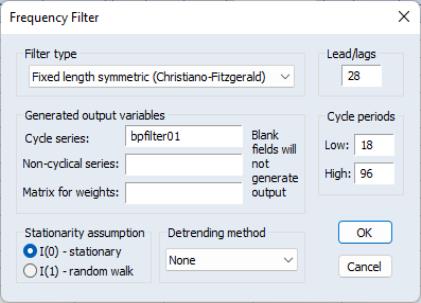
Both of the CF filters (symmetric and asymmetric) provide you with additional options for handling trending data.
The first setting involves the . For both of the CF, you will need to specify whether the series is assumed to be an I(0) covariance stationary process or an I(1) unit root process.
Lastly, you will select a using the dropdown. For a covariance stationary series, you may choose to demean or detrend the data prior to applying the filters. Alternatively, for a unit root process, you may choose to demean, detrend, or remove drift using the adjustment suggested by Christiano and Fitzgerald (2003).
Note that, as the name suggests, the full sample filter uses all of the observations in the sample, so that the option is not relevant. Similarly, detrending the data is not an option when using the BK fixed length symmetric filter. The BK filter removes up to two unit roots (a quadratic deterministic trend) in the data so that detrending has no effect on the filtered series.
The Filter Output
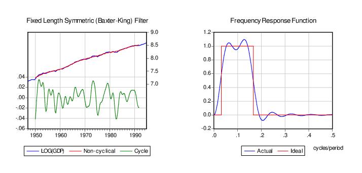
Here, we depict the output from the Baxter-King filter using the series LOG(GDP) in the workfile “Bpf.WF1”. The results were produced by selecting from the main series menu and clicking on to accept the default settings. (We have added grid lines to the graph to make it easier to see the cyclical behavior). The left panel depicts the original series, filtered series, and the non-cyclical component (difference between the original and the filtered).
For the BK and CF fixed length symmetric filters, EViews plots the frequency response function

representing the extent to which the filtered series “responds” to the original series at frequency

. At a given frequency

,

indicates the extent to which a moving average raises or lowers the variance of the filtered series relative to that of the original series. The right panel of the graph depicts the function. Note that the horizontal axis of a frequency response function is always in the range 0 to 0.5, in units of cycles per duration. Thus, as depicted in the graph, the frequency response function of the ideal band-pass filter for periodicities

will be one in the range
.
The frequency response function is not drawn for the CF time-varying filter since these filters vary with the data and observation number. If you wish to plot the frequency response function for a particular observation, you will have to save the weight matrix and then evaluate the frequency response in a separate step. The example program BFP02.PRG and subroutine FREQRESP.PRG illustrate the steps in computing of gain functions for time-varying filters at particular observations.
The Weight Matrix
For time-invariant (fixed-length symmetric) filters, the weight matrix is of dimension

where

is the user-specified lag length order. For these filters, the weights on the leads and the lags are the same, so the returned matrix contains only the one-sided weights. The filtered series can be computed as:
For time-varying filters, the weight matrix is of dimension

where

is the number of non-missing observations in the current sample. Row

of the matrix contains the weighting vector used to generate the

-th observation of the filtered series where column

contains the weight on the

-th observation of the original series:
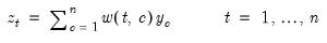 | (11.107) |
where

is the filtered series,

is the original series and

is the

element of the weighting matrix. By construction, the first and last rows of the weight matrix will be filled with missing values for the symmetric filter.