Switching Views
Once you have estimated your VAR, EViews offers a variety of views for examining your results.
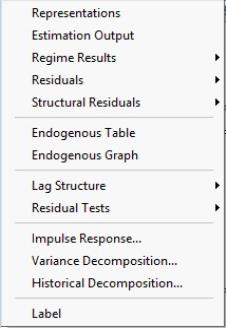
Most of these routines are familiar tools for working with a VAR. You may, for example, examine plots for your estimated equation, examine the of your VAR, or use the submenu to examine properties of your residuals.
Since the presence of switching and multiple regimes creates a few wrinkles, we offer a few comments on select views.
Regime Results
EViews offers specialized tools for examining the regime transition results and predicted regime probabilities.
Transition Results
To display the transition results dialog, select EViews offers to display different types of output: , , and .
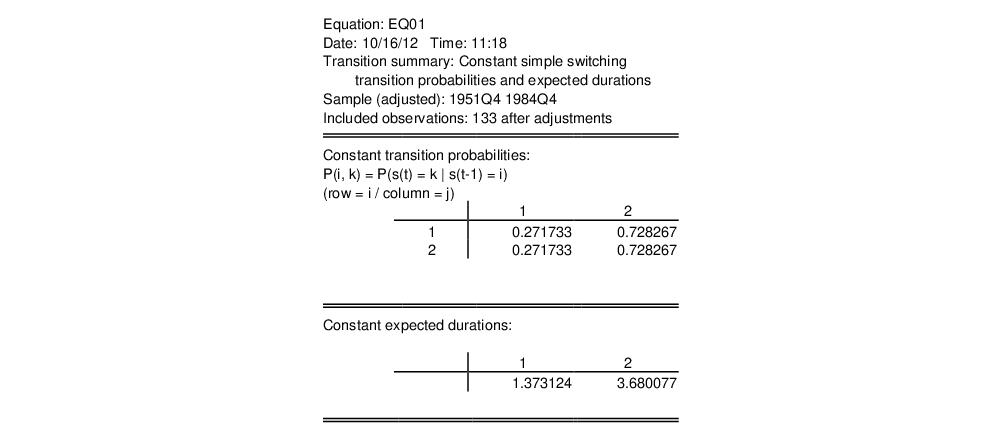
The default display shows a table containing both the transition matrix and the expected durations (Kim and Nelson, 1999, p. 71-72) implied by the transition matrix. For example,
Here, we see results from the simple switching model with constant transition probabilities. Note that since the model assumes simple switching, the probabilities of being in regime 1 and regime 2 (approximately 0.27 and 0.73, respectively) do not depend on the origin state. These probabilities imply that the expected duration in a regime is roughly 1.37 quarters in regime 1 and 3.68 quarters in regime 2.
In models with varying transition probabilities, the transition probability summary will instead show the means and standard deviations of the transition probabilities and the expected durations.
The latter two output type choices may prove useful in models with time-varying transition probabilities:
• Selecting allows you to see the transition matrix in every period. You will be offered a choice of displaying the transition probabilities in (default), , or form.
The display shows a multiple graph showing each transition probability. For purposes of this display simple switching models are treated as restricted Markov switching models. Thus, a two-regime switching model will always show four separate graphs, one for each transition. Note that for constant transition probability models, each graph will be a straight line.
The display shows the same results in spreadsheet format while the form displays results for each period in a table form similar to that used in the summary display. For constant probability models, the spreadsheet format will contain identical rows and the table form will show a single transition matrix.
• Lastly, you may display the associated with the transition matrix in each period. The results may be displayed in (default), , or form. For constant probability models, the table form will only show the single set of expected durations.
Regime Probabilities
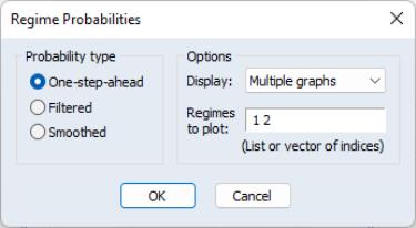
To display the estimated regime probabilities select
EViews offers a choice between the , , and probabilities. For simple switching models without AR terms, the filtered and smoothed results are the same. In addition, you may display the results in , in a , or in form.
For graphical output you may also select which regimes to plot by entering the corresponding indices in the edit field. While the default is to show the probabilities for all regimes, you may use the edit field to remove redundant probabilities or to focus on a specific regime of interest.
Residuals and Structural Residuals Diagnostics
The and submenus provides various views of the residuals and associated fitted values. The fits and residuals are formed by taking expectations using regime specific values and the one-step ahead regime probabilities. The standardized residuals are computed similarly with the regime specific residuals scaled by the estimate of the regime standard error prior to forming the expectations (Maheu and McCurdy, 2000).
EViews offers select diagnostics in the submenu. Some care should be taken in the use of these views. Maheu and McCurdy note, for example, that the standardized residuals may be used in Ljung-Box tests, but urge caution in interpreting the results since asymptotic results using these residuals are not available.
Regime Specific Lagged Endogenous


