Working with Threshold Equations
The threshold equation produced by the EViews threshold estimation procedure is, in essence, a linear regression model with regime dummies on some or all of the variables. For the most part, views and procs will work as in standard models, though some care should be taken in interpreting results.
We describe below the basics of working with your threshold equation, highlighting views and procs for which there are important differences, along with threshold specific tools.
Estimation Output
Suppose we estimate a two-regime threshold regression model with an AR(11) in each regime and model selection over threshold dependent variable lags from -1 to -5 using the LYNX_TRANSF series in the “terasvirta_lynx.WF1” example workfile.
The top part of the output shows equation specification information.
In addition to the usual dependent variable, method, date, and sample information, EViews displays information about the threshold specification. Here we see that the threshold value was found using the fixed number (one) of sequentially determined thresholds. Since we instructed EViews to perform model selection using 1 to 5 lags of the LYNX_TRANSF series, EViews displays the names of all of the candidate series. Lastly, EViews displays the selected threshold variable and the estimated threshold value.
Some comments on the reported threshold value are in order. Recall that the threshold values are only identified up to an interval defined by adjacent values of the sorted threshold variable (Tsay, 1989). For purposes of display, EViews reports the observed value of the threshold variable at the beginning of a regime, truncated to a more readable form, while ensuring that the representation satisfies the threshold inequalities.
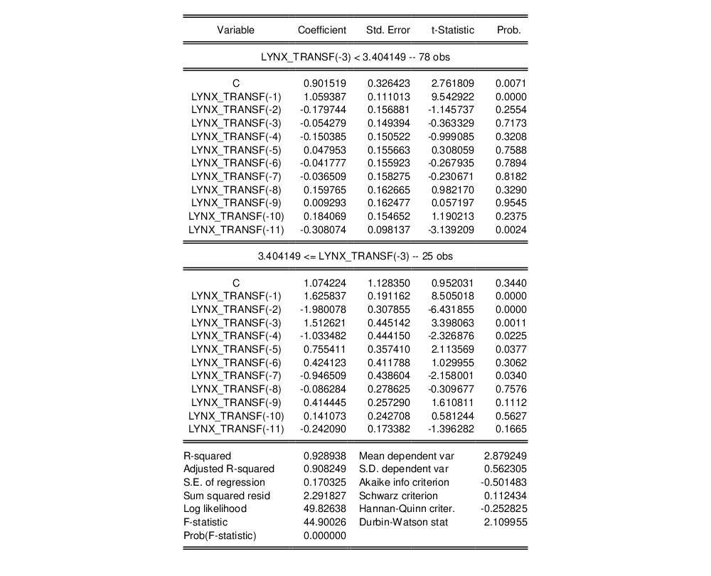
The middle part of the output labels displays coefficient values and associated statistics for each regime. The bottom portion of the output contains the usual summary statistics.
Most of the summary statistics are self-explanatory. We do note that the

-square, the
F-statistic, and the corresponding probability are all based on a comparison with the fully restricted, no threshold, constant only model.
Equation Views and Procs
Not surprisingly, the available views and procs for threshold equations parallel those in breakpoint least squares regression, with some additions as described below. Additionally we address some subtle and not-so-subtle issues that you should bear in mind when working with the familiar routines.
Criteria Graph and Table
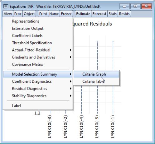
If you select from an estimated threshold equation you will be offered a choice of displaying a or a :
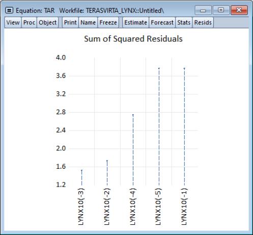
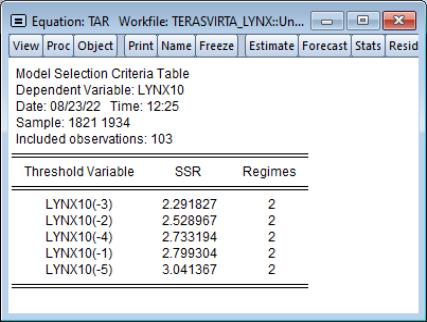
These two views display the model selection criteria used to select the threshold variable in a line plot or a table, ordered by the selection criterion.
For example, the criteria graph for this equation is shown below:
In this figure, the threshold variable whose model has the lowest AIC is clearly visible on the left of the graph.
Here, we see the same set of results in table form. This view also includes information about the common sample used for model selection estimation, and the number of regimes employed for each candidate model.
Representations View
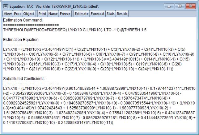
The representations view () shows the expanded equation specification, which combines the coefficients from different regimes with the threshold variable and limits and various inequalities into a single equation.
Note that estimating this single equation specification via ordinary least squares will produce the same coefficients as the estimated threshold model.
Threshold Specification
The threshold specification view displays more detailed information about the threshold variable, values, along with information about the method of selecting the number of thresholds. To display this view, click on from the equation menu.
The top portion of the output displays information about the threshold and threshold values:
The detailed information on the threshold values includes the actual data value corresponding to the break (in this case 3.40414924921), the actual data value for the next highest data value (here 3.39984671271), and the truncated value EViews uses for display and representation purposes (3.404149). (Note that any value between the lower adjacent data value and the threshold data value would produce the same observed fit).
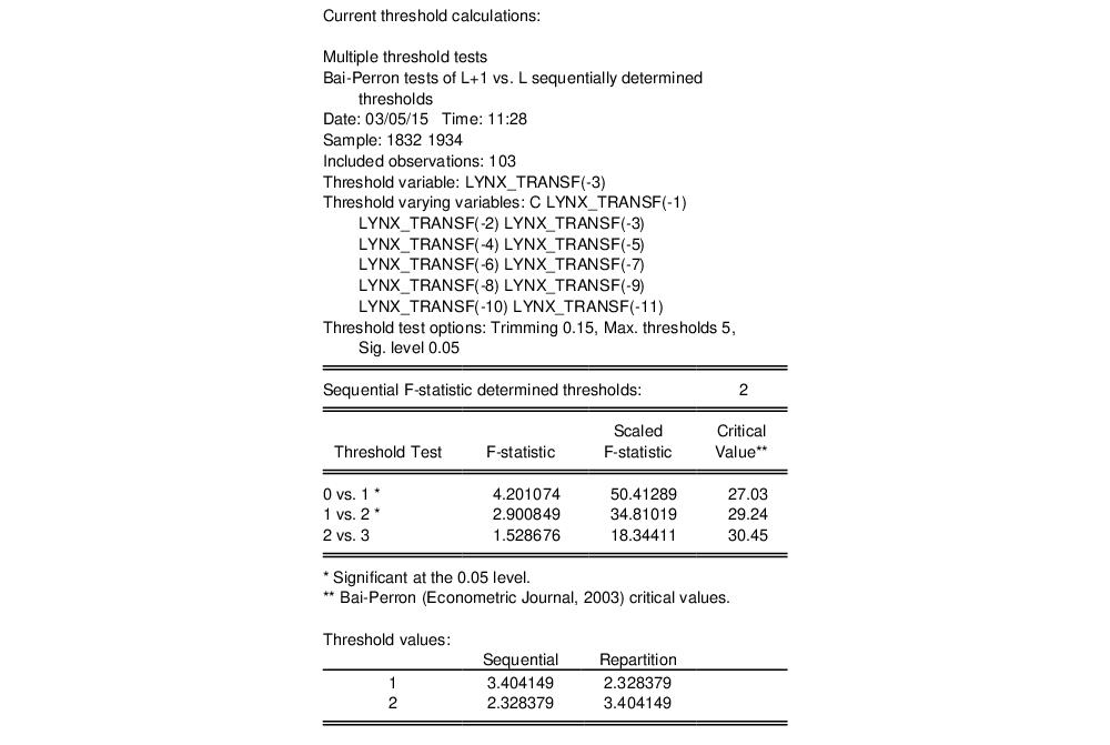
The lower portion of the output displays calculations used in determining the thresholds:
In this case, EViews displays the results for sequentially determined thresholds using the Bai-Perron Sup-F test statistics. We caution again that since this TAR specification contains lagged endogenous variables, that the conditions required for distributional results is violated (Hansen, 1999; Hansen, 2000).
Omitted and Redundant Variables Testing
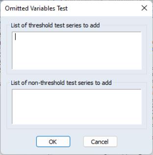
The omitted variables test (), requires the specification of regime-specific or common variables:
Simply enter the variables you wish to add in the appropriate edit field.
Alternately, the redundant variables test will prompt you to enter variables from the original specification that you wish to drop.
We point out that these tests are performed conditionally on the thresholds identified in the estimation step. EViews will use the threshold variables and values previously determined and perform the test on the conditional linear specification. This may not be the test you wish to perform.
Forecasting
Static or one-step ahead forecasting from a TR estimated equation is straightforward, and involves conditioning on the observed regressors, including any lagged endogenous and computing the forecast.
For TAR and other models with lagged endogenous variables,

-step ahead nonlinear dynamic forecasting is considerably trickier (see, for example the discussion in Potter 1999, or Tong and Lim, 1980 who distinguish between the “eventual forecasting function” and the

-step ahead forecasts). For dynamic threshold regression models, EViews computes forecasts by stochastic simulation with the forecasts and forecast standard errors obtained from the sample average and standard deviation of the simulated values.
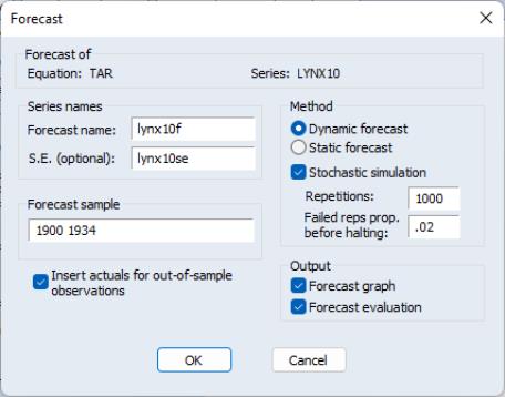
To perform the forecast simulation, click on the button on the equation toolbar or select from the equation menu to display the dialog:
Most of this dialog should be familiar. Note, however, that under the section are two new edit fields for controlling the stochastic simulation, one for the number of , and the second for the .
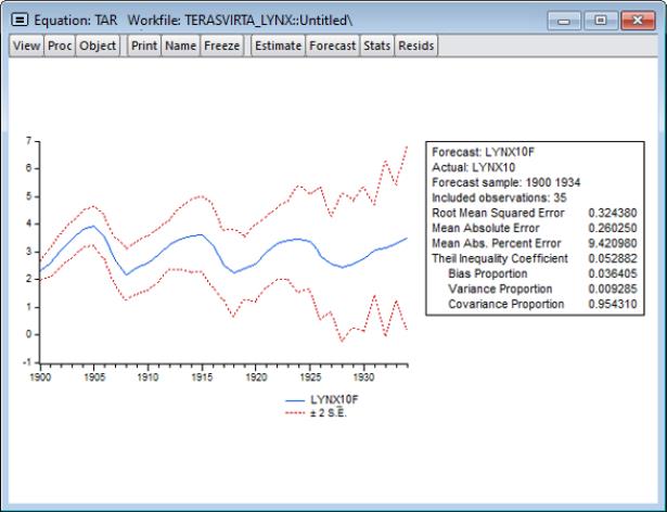
Change the settings as desired and click on to continue. Here we tell EViews we wish to compute the simulated dynamic forecasts from 1900 to 1934. EViews displays the results of the forecast along with evaluation statistics:
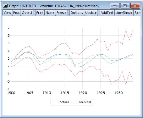
We may use the saved values of the forecast and standard error series to show a comparison with the actuals. First, display a graph containing the series using the command:
plot lynx_transf lynx_transfcst lynx_transfcst+2*lynx_transfse lynx_transfcst-2*lynx_transfse
After a bit of editing to change line colors, patterns, and legend entries, we have:


 -square, the F-statistic, and the corresponding probability are all based on a comparison with the fully restricted, no threshold, constant only model.

 -step ahead nonlinear dynamic forecasting is considerably trickier (see, for example the discussion in Potter 1999, or Tong and Lim, 1980 who distinguish between the “eventual forecasting function” and the
  -step ahead forecasts). For dynamic threshold regression models, EViews computes forecasts by stochastic simulation with the forecasts and forecast standard errors obtained from the sample average and standard deviation of the simulated values.