EViews Help: Applications

For illustrative purposes, we provide a demonstration of how to carry out some other specification tests in EViews. For brevity, the discussion is based on commands, but most of these procedures can also be carried out using the menu system.

The F-statistics reported in the Chow tests have an F-distribution only if the errors are independent and identically normally distributed. This restriction implies that the residual variance in the two subsamples must be equal.

Suppose now that we wish to compute a Wald statistic for structural change with unequal subsample variances. Denote the parameter estimates and their covariance matrix in subsample

and

for

. Under the assumption that

and

are independent normal random variables, the difference

has mean zero and variance

. Therefore, a Wald statistic for the null hypothesis of no structural change and independent samples can be constructed as:

which has an asymptotic

distribution with degrees of freedom equal to the number of estimated parameters in the

vector.

To carry out this test in EViews, we estimate the model in each subsample and save the estimated coefficients and their covariance matrix. For example, consider the quarterly workfile of macroeconomic data in the workfile “Coef_test2.WF1” (containing data for 1947q1–1994q4) and suppose wish to test whether there was a structural change in the consumption function in 1973q1. First, estimate the model in the first sample and save the results by the commands:

The first line declares the coefficient vector, B1, into which we will place the coefficient estimates in the first sample. Note that the equation specification in the third line explicitly refers to elements of this coefficient vector. The last line saves the coefficient covariance matrix as a symmetric matrix named V1. Similarly, estimate the model in the second sample and save the results by the commands:

To compute the Wald statistic, use the command:

The Wald statistic is saved in the

matrix named WALD. To see the value, either double click on WALD or type “show wald”. You can compare this value with the critical values from the

distribution with 2 degrees of freedom. Alternatively, you can compute the p-value in EViews using the command:

The p-value is saved as a scalar named WALD_P. To see the p-value, double click on WALD_P or type “show wald_p”. The WALD statistic value of 53.1243 has an associated p-value of 2.9e-12 so that we decisively reject the null hypothesis of no structural change.

A widely used class of tests in econometrics is the Hausman test. The underlying idea of the Hausman test is to compare two sets of estimates, one of which is consistent under both the null and the alternative and another which is consistent only under the null hypothesis. A large difference between the two sets of estimates is taken as evidence in favor of the alternative hypothesis.

Hausman (1978) originally proposed a test statistic for endogeneity based upon a direct comparison of coefficient values. Here, we illustrate the version of the Hausman test proposed by Davidson and MacKinnon (1989, 1993), which carries out the test by running an auxiliary regression.

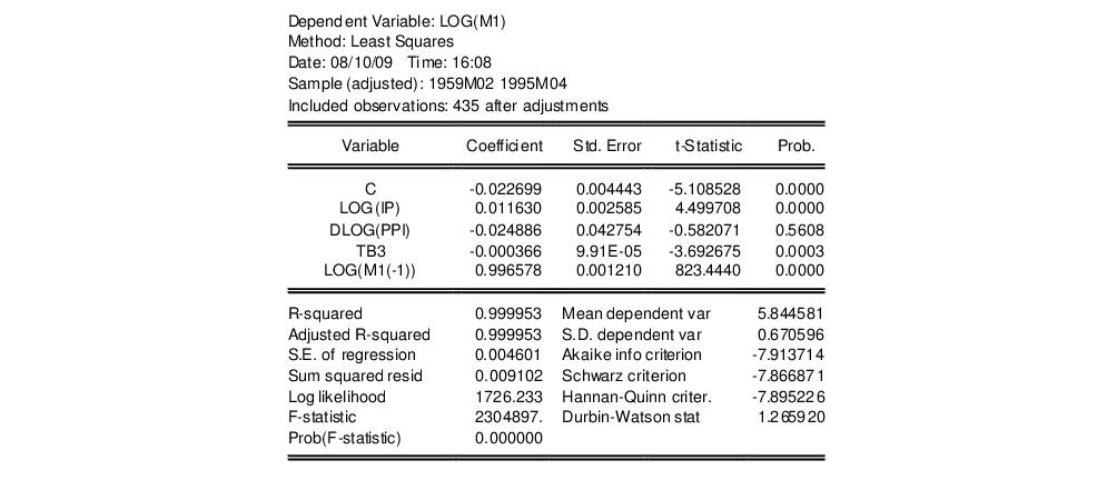
The following equation in the “Basics.WF1” workfile was estimated by OLS:

Suppose we are concerned that industrial production (IP) is endogenously determined with money (M1) through the money supply function. If endogeneity is present, then OLS estimates will be biased and inconsistent. To test this hypothesis, we need to find a set of instrumental variables that are correlated with the “suspect” variable IP but not with the error term of the money demand equation. The choice of the appropriate instrument is a crucial step. Here, we take the unemployment rate (URATE) and Moody’s AAA corporate bond yield (AAA) as instruments.

To carry out the Hausman test by artificial regression, we run two OLS regressions. In the first regression, we regress the suspect variable (log) IP on all exogenous variables and instruments and retrieve the residuals:

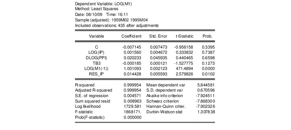
Then in the second regression, we re-estimate the money demand function including the residuals from the first regression as additional regressors. The result is:

If the OLS estimates are consistent, then the coefficient on the first stage residuals should not be significantly different from zero. In this example, the test rejects the hypothesis of consistent OLS estimates at conventional levels.

Note that an alternative form of a regressor endogeneity test may be computed using the Regressor Endogeneity Test view of an equation estimated by TSLS or GMM (see “Regressor Endogeneity Test”).

Most of the tests discussed in this chapter are nested tests in which the null hypothesis is obtained as a special case of the alternative hypothesis. Now consider the problem of choosing between the following two specifications of a consumption function:

for the variables in the workfile “Coef_test2.WF1”. These are examples of non-nested models since neither model may be expressed as a restricted version of the other.

The J-test proposed by Davidson and MacKinnon (1993) provides one method of choosing between two non-nested models. The idea is that if one model is the correct model, then the fitted values from the other model should not have explanatory power when estimating that model. For example, to test model

against model

, we first estimate model

and retrieve the fitted values:

The second line saves the fitted values as a series named CS2. Then estimate model

including the fitted values from model

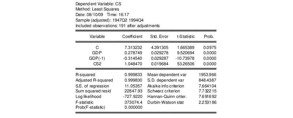
. The result is:

Then estimate model

including the fitted values from model

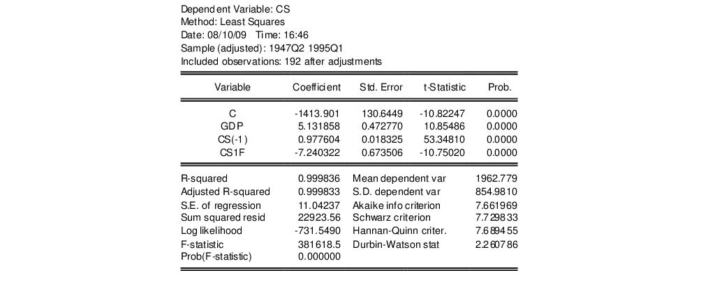
. The results of this “reverse” test regression are given by:

In this example, we reject both specifications, against the alternatives, suggesting that another model for the data is needed. It is also possible that we fail to reject both models, in which case the data do not provide enough information to discriminate between the two models.