Impulse Response Functions
Consider a system of

time series of length

. If the system is modeled as a vector autoregressive (VAR) process of order

, the data generating process (DGP) for the system is written as:
 | (46.1) |
where

and

are

vectors,

are

matrices, and

, where

is a

covariance matrix.
This properties of this model and various approaches to estimation are described in
“Vector Autoregression (VAR) Models”.
Traditional VAR IR
Traditionally, impulse response functions are estimated from the Wold decomposition of an estimated VAR model.
Construction of the impulse response functions proceeds in two steps. In the first step, a VAR model is specified and estimated. In the second, the estimated VAR coefficients are inverted to derive the Wold form (a linear function of the innovations

) which provides the coefficient weights on the innovations in the impulse response.
Formally, impulse response paths to shocks in

are based on the recursion
 | (46.2) |
for

and

,

, and

is longest response horizon of interest.
The (
i,
j)-th element of

is the response of variable
i at horizon step
h to a unit shock in variable
j. Thus, the responses for all of the variables to a unit shock at horizon

are obtained by post-multiplying the matrix

by the corresponding unit impulse vector.
Given an estimated VAR, the IR estimates

are computed by simply replacing

with the corresponding estimates

.
Stacking the estimators for each

vertically, the estimated full impulse response path is given by:
If the innovations

are contemporaneously uncorrelated (

is diagonal), it is easy to interpret the impulse responses: an impulse in the
j-th error is equivalent to a shock to the
j-th endogenous variable, which produces a response in all of the variables at different horizons.
The innovations, however, are typically correlated. We may think of correlation in the errors as emanating from an unmodeled common component. Given this commonality, it becomes conceptually difficult to interpret an impulse in the j-th error that is not accompanied by shocks in related variables.
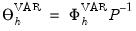
To aid in interpretation, it is common to consider the impulse response path associated with orthogonalized innovations. Suppose that there exists a transformation

such that the innovations are uncorrelated:
 | (46.3) |
where

is a
diagonal covariance matrix.
Note that
Equation (46.1) may be written in terms of orthogonal innovations

 | (46.4) |
so that the impulse responses may be written in terms of shocks to

. It follows that the impulse responds with respect to innovations in

are governed by
 | (46.5) |
with the (
i,
j)-th element of

giving the response of variable
i at horizon step
h to a unit shock in the
j-th orthogonal innovation.
In practice,

is computed using

from above and

computed using results from the VAR if estimation of

is required.
The full, estimated impulse response path is given by
 | (46.6) |
Local Projection
The traditional VAR approach to impulse response estimation has both practical and theoretical shortcomings. In particular, the Wold decomposition can be difficult to derive, and may not exist, more likely in cases where the VAR is cointegrated. Further, impulse response functions derived from this method are justified only when the estimated VAR model coincides with the true DGP.
An alternative approach proposes the estimation of impulse responses via local projections (Jordà, 2005). The local projection (LP) technique is agnostic about the true DGP, and remains valid even when the Wold decomposition is undefined. LP defines the response function to a shock in the i-th variable as the difference between two forecasts:
 | (46.7) |
for

, where the operator

denotes the best mean squared error predictor and
is the matrix of its lags.
Since this definition reduces the estimation of the impulse response path to a linear forecast, Jordà (2005) shows that
Equation (46.1) may be estimated as a projection of

onto the linear space generated by
.
Sequential Estimation
Consider the

local linear projections
 | (46.8) |
for
. By construction, the estimated slopes

may be interpreted as the response of

to a reduced-form disturbance in period

, and we may define the impulse response estimators,
 | (46.9) |
The full, estimated impulse response path for reduced-form impulses is then given by:
 | (46.10) |
with the normalization

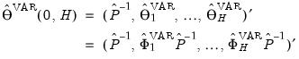
. The estimates of orthogonalized impulse responses are given by
 | (46.11) |
and the full, estimated impulse response path for orthogonalized impulses is
 | (46.12) |
Joint Estimation
Instead of estimating the impulse response path sequentially, we may estimate the response at all horizon steps,

, simultaneously. Define the following matrices:
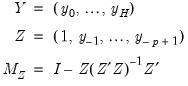 | (46.13) |
The joint local projection estimator of the impulse response path to a reduced-form disturbance in period t is then:
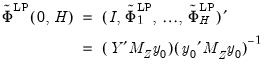 | (46.14) |
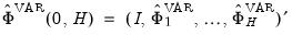
and the full impulse response path resulting from structural shocks may be written as:
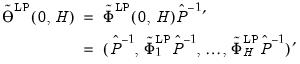 | (46.15) |
Nonlinear Estimation
An appealing feature of impulse response paths derived via local projections is that they lend themselves to nonlinear estimation. For instance, these methods are well-suited to models with complicated switching structures, as in the study of impulse response effects under different policies of Ahmed and Cassou (2016). Consider the following binary regime setup:
 | (46.16) |
for

where
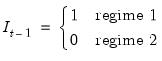 | (46.17) |
Given sequential estimates of the

and

from this set of equations, the impulse response paths for the two regimes are given by,
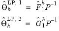 | (46.18) |
and the full paths are
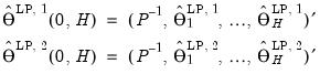 | (46.19) |
We may generalize this result to the case of more than one regime defined by categorical variables and can derive corresponding expressions for joint nonlinear estimation.
 is
is  ,
,  is
is  , and
, and  is
is