Structuring a Workfile
You may, at any time, change the underlying structure of an existing workfile or workfile page by applying structuring information. We call this process structuring a workfile. There are four primary types of structuring information that you may provide:
• regular date descriptions.
• variables containing observation identifiers for dated data.
• variables containing observation identifiers for cross-section data.
• variables containing observation identifiers defining a panel data structure.
The ability to structure your data is an important feature, and we will explore structured workfiles at some length.
Types of Structured Data
Before describing the process of structuring a workfile or workfile page, we define some concepts related to the various data structures.
Regular and Irregular Frequency Data
As the name suggests,
regular frequency data arrive at regular intervals (daily, monthly, annually, etc.). Standard macroeconomic data such as quarterly GDP or monthly housing starts are examples of regular frequency data. This type of data is introduced in
“Creating a Workfile by Describing its Structure”.
Unlike regular frequency data, Irregular frequency data do not arrive in a precisely regular pattern. An important example of irregular data is found in stock and bond prices, where the presence of missing days due to holidays and other market closures means that the data do not follow a regular daily (7- or 5-day) frequency.
The most important characteristic of regular data is that there are no structural gaps in the data—all observations in the specified frequency exist, even if there are missing values that are not observed. Alternatively, irregular data allow for gaps between successive observations in the given regular frequency. This is a subtle distinction, but has important consequences for lag processing.
The distinction is best illustrated by an example. Suppose that we are working with a daily calendar and that we have two kinds of data: data on bond prices (BOND), and data on temperature in Los Angeles in Farenheit (TEMP):
| | | |
12/21 | Sun | <mkt.closed> | 68 |
12/22 | Mon | 102.78 | 70 |
12/23 | Tues | 102.79 | NA |
12/24 | Wed | 102.78 | 69 |
12/25 | Thurs | <mkt.closed> | 68 |
12/26 | Fri | 102.77 | 70 |
Notice that in this example, the bond price is not available on 12/21 and 12/25 (since the market was closed), and that the temperature reading was not available on 12/23 (due to equipment malfunction).
Typically, we would view the TEMP series as following a 7-day regular daily frequency with a missing value for 12/23. The key feature of this interpretation is that the day 12/23 exists, even though a temperature reading was not taken on that day. Most importantly, this interpretation implies that the lagged value of TEMP on 12/24 (the previous day’s TEMP value) is NA.
In contrast, most analysts would view BOND prices as following an irregular daily frequency in which days involving market closures do not exist. Under this interpretation, we would remove weekends and holidays from the calendar so that the bond data would be given by:
| | |
12/22 | Mon | 102.78 |
12/23 | Tue | 102.79 |
12/24 | Wed | 102.78 |
12/26 | Fri | 102.77 |
The central point here is that lags are defined differently for regular and irregular data. Given a regular daily frequency, the lagged value of BOND on 12/26 would be taken from the previous day, 12/25, and would be NA. Given the irregular daily frequency, the lagged value on 12/26 is taken from the previous observation, 12/24, and would be 102.78. In defining an irregular calendar, we explicitly skip over the structural gaps created by market closure.
You may always convert irregular frequency data into regular frequency data by adding any observations required to fill out the relevant calendar. If, for example, you have 7-day irregular data, you may convert it to a regular frequency by adding observations with IDs that correspond to any missing days.
Undated Data with Identifiers
Perhaps the simplest data structure involves undated data. We typically refer to these data as cross-section data. Among the most common examples of cross-section data are state data taken at a single point in time:
| | | |
1 | 2002 | Alabama | .000 |
2 | 2002 | Arkansas | .035 |
3 | 2002 | Arizona | .035 |
... | 2002 | ... | ... |
50 | 2002 | Wyoming | .010 |
Here we have an alphabetically ordered dataset with 50 observations on state tax rates. We emphasize the point that these data are undated since the common YEAR of observation does not aid in identifying the individual observations.
These cross-section data may be treated as an unstructured dataset using the default integer identifiers 1 to 50. Alternatively, we may structure the data using the unique values in STATE as identifiers. These state name IDs will then be used when referring to or labeling observations. The advantages of using the state names as identifiers should be obvious—comparing data for observation labeled “Arizona” and “Wyoming” is much easier than comparing data for observations “3” and “50”.
One last comment about the ordering of observations in cross-section data. While we can (and will) define the lag observation to be that “preceding” a given observation, such a definition is sensitive to the arbitrary ordering of our data, and may not be meaningful. If, as in our example, we order our states alphabetically, the first lag of “Arkansas” is taken from the “Arizona” observation, while if we order our observations by population, the lag of “Arkansas” will be the data for “Utah”.
Panel Data
Some data involve observations that possess both cross-section (group) and within-cross-section (cell) identifiers. We will term these to be panel data. Many of the previously encountered data structures may be viewed as a trivial case of panel data involving a single cross-section.
To extend our earlier example, suppose that instead of observing the cross-section state tax data for a single year, we observe these rates for several years. We may then treat an observation on any single tax rate as having two identifiers: a single identifier for STATE (the group ID), and an identifier for the YEAR (the cell ID). The data for two of our states, “Kansas” and “Kentucky” might look like the following:
| | | |
... | ... | ... | ... |
80 | Kansas | 2001 | .035 |
81 | Kansas | 2002 | .037 |
82 | Kansas | 2003 | .036 |
83 | Kentucky | 2001 | .014 |
84 | Kentucky | 2003 | .016 |
... | ... | ... | ... |
We emphasize again that identifiers must uniquely determine the observation. A corollary of this requirement is that the cell IDs uniquely identify observations within a group. Note that requiring cell IDs to be unique within a group does not imply that the cell IDs are unique. In fact, cell ID values are usually repeated across groups; for example, a given YEAR value appears in many states since the tax rates are generally observed in the same years.
If we observe repeated values in the cell identifiers within any one group, we must either use a different cell identifier, or we must redefine our notion of a group. Suppose, for example, that Kansas changed its tax rate several times during 2002:
| | | | | |
... | ... | ... | ... | ... | ... |
80 | Kansas | 2001 | 1 | 1 | .035 |
81 | Kansas | 2002 | 2 | 1 | .037 |
82 | Kansas | 2002 | 3 | 2 | .038 |
83 | Kansas | 2002 | 4 | 3 | .035 |
84 | Kansas | 2003 | 5 | 1 | .036 |
85 | Kentucky | 2001 | 1 | 1 | .014 |
86 | Kentucky | 2003 | 2 | 2 | .016 |
... | ... | ... | ... | ... | ... |
In this setting, YEAR would not be a valid cell ID for groups defined by STATE, since 2002 would be repeated for STATE=“Kansas”.
There are a couple of things we may do. First, we may simply choose a different cell identifier. We could, for example, create a variable containing a default integer identifier running within each cross-section. For example, the newly created variable CELL_ID1 is a valid cell ID since it provides each “Kansas” and “Kentucky” observation with a unique (integer) value.
Alternately, we may elect to subdivide our groups. We may, for example, choose to use both STATE and YEAR as the group identifier. This specification defines a group for each unique STATE and YEAR combination (e.g. — observations for which STATE=“Kansas” and YEAR=“2002” would comprise a single group). Given this new group definition, we may use either CELL_ID1 or CELL_ID2 as cell identifiers since they are both unique for each STATE and YEAR group. Notice that CELL_ID2 could not have been used as a valid cell ID for STATE groups since it does not uniquely identify observations within Kansas.
While it may at first appear to be innocuous, the choice between creating a new variable or redefining your groups has important implications (especially for lag processing). Roughly speaking, if you believe that observations within the original groups are closely “related”, you should create a new cell ID; if you believe that the subdivision creates groups that are more alike, then you should redefine your group IDs.
In our example, if you believe that the observations for “Kansas” in “2001” and “2002” are both fundamentally “Kansas” observations, then you should specify a new cell ID. On the other hand, if you believe that observations for “Kansas” in “2002” are very different from “Kansas” in “2001”, you should subdivide the original “Kansas” group by using both STATE and YEAR as the group ID.
Lags, Leads, and Panel Structured Data
Following convention, the observations in our panel dataset are always stacked by cross-section. We first collect the observations by cross-section and sort the cell IDs within each cross-section. We then stack the cross sections on top of one another, with the data for the first cross-section followed by the data for the second cross-section, the second followed by the third, and so on.
The primary impact of this data arrangement is its effect on lag processing. There are two fundamental principles of lag processing in panel data structures:
• First, lags and leads do not cross group boundaries, so that they never use data from a different group.
• Second, lags and leads taken within a cross-section are defined over the sorted values of the cell ID. This implies that lags of an observation are always associated with lower value of the cell ID, and leads always involve a higher value (the first lag observation has the next lowest value and the first lead has the next highest value).
Let us return to our original example with STATE as the group ID and YEAR as the cell ID, and consider the values of TAXRATE, TAXRATE(-1), and TAXRATE(1). Applying the two rules for panel lag processing, we have:
| | | | | |
... | ... | ... | ... | ... | ... |
80 | Kansas | 2001 | .035 | NA | .037 |
81 | Kansas | 2002 | .037 | .035 | .036 |
82 | Kansas | 2003 | .036 | .037 | NA |
83 | Kentucky | 2001 | .014 | NA | .016 |
84 | Kentucky | 2003 | .016 | .014 | NA |
... | ... | ... | ... | | |
Note in particular, that the lags and leads of TAXRATE do not cross the group boundaries; the value of TAXRATE(-1) for Kentucky in 2001 is an NA since the previous value is from Kansas, and the value TAXRATE(1) for Kansas in 2003 is NA is the next value is from Kentucky.
Next, consider an example where we have invalid IDs since there are duplicate YEAR values for Kansas. Recall that there are two possible solutions to this problem: (1) creating a new cell ID, or (2) redefining our groups. Here, we see why the choice between using a new cell ID or subdividing groups has important implications for lag processing. First, we may simply create a new cell ID that enumerates the observations in each state (CELL_ID1). If we use CELL_ID1 as the cell identifier, we have:
| | | | | |
... | ... | ... | ... | ... | |
80 | Kansas | 2001 | 1 | .035 | NA |
81 | Kansas | 2002 | 2 | .037 | .035 |
82 | Kansas | 2002 | 3 | .038 | .037 |
83 | Kansas | 2002 | 4 | .035 | .038 |
84 | Kansas | 2003 | 5 | .036 | .035 |
85 | Kentucky | 2001 | 1 | .014 | NA |
86 | Kentucky | 2003 | 2 | .016 | .014 |
... | ... | ... | ... | ... | |
Note that the only observations for TAXRATE(-1) that are missing are those at the “seams” joining the cross-sections.
Suppose instead that we elect to subdivide our STATE groupings by using both STATE and YEAR to identify a cross-section, and we create CELL_ID2 which enumerates the observations in each cross-section. Thus, each group is representative of a unique STATE-YEAR pair, and the cell ID indexes observations in a given STATE for a specific YEAR. The TAXRATE(-1) values are given in:
| | | | | |
... | ... | ... | ... | ... | ... |
80 | Kansas | 2001 | 1 | .035 | NA |
81 | Kansas | 2002 | 1 | .037 | NA |
82 | Kansas | 2002 | 2 | .038 | .037 |
83 | Kansas | 2002 | 3 | .035 | .038 |
84 | Kansas | 2003 | 1 | .036 | NA |
85 | Kentucky | 2001 | 1 | .014 | NA |
86 | Kentucky | 2003 | 2 | .016 | .014 |
... | ... | ... | ... | ... | ... |
Once again, the missing observations for TAXRATE(-1) are those that span cross-section boundaries. Note however, that since the group boundaries are now defined by STATE and YEAR, there are more seams and TAXRATE(-1) has additional missing values.
In this simple example, we see the difference between the alternate approaches for handling duplicate IDs. Subdividing our groups creates additional groups, and additional seams between those groups over which lags and leads are not processed. Accordingly, if you wish your lags and leads to span all of the observations in the original groupings, you should create a new cell ID to be used with the original group identifier.
Types of Panel Data
Panel data may be characterized in a variety of ways. For purposes of creating panel workfiles in EViews, there are several concepts that are of particular interest.
Dated vs. Undated Panels
We characterize panel data as dated or undated on the basis of the cell ID. When the cell ID follows a frequency, we have a dated panel of the given frequency. If, for example, our cell IDs are defined by a variable like YEAR, we say we have an annual panel. Similarly, if the cell IDs are quarterly or daily identifiers, we say we have a quarterly or daily panel.
Alternatively, an undated panel uses group specific default integers as cell IDs; by default the cell IDs in each group are usually given by the default integers (1, 2, ...).
Regular vs. Irregular Dated Panels
Dated panels follow a regular or an irregular frequency. A panel is said to be a regular frequency panel if the cell IDs for every group follow a regular frequency. If one or more groups have cell ID values which do not follow a regular frequency, the panel is said to be an irregular frequency panel.
One can convert an irregular frequency panel into a regular frequency panel by adding observations to remove gaps in the calendar for all cross-sections. Note that this procedure is a form of internal balancing (see
“Balanced vs. Unbalanced Panels” below) which uses the calendar to determine which observations to add instead of using the set of cell IDs found in the data.
See
“Regular and Irregular Frequency Data” for a general discussion of these topics.
Balanced vs. Unbalanced Panels
If every group in a panel has an identical set of cell ID values, we say that the panel is fully balanced. All other panel datasets are said to be unbalanced.
In the simplest form of balanced panel data, every cross-section follows the same regular frequency, with the same start and end dates—for example, data with 10 cross-sections, each with annual data from 1960 to 2002. Slightly more complex is the case where every cross-section has an identical set of irregular cell IDs. In this case, we say that the panel is balanced, but irregular.
We may balance a panel by adding observations to the unbalanced data. The procedure is quite simple—for each cross-section or group, we add observations corresponding to cell IDs that are not in the current group, but appear elsewhere in the data. By adding observations with these “missing” cell IDs, we ensure that all of the cross-sections have the same set of cell IDs.
To complicate matters, we may partially balance a panel. There are three possible methods—we may choose to balance between the starts and ends, to balance the starts, or to balance the ends. In each of these methods, we perform the procedure for balancing data described above, but with the set of relevant cell IDs obtained from a subset of the data. Performing all three forms of partial balancing is the same as fully balancing the panel.
Balancing data between the starts and ends involves adding observations with cell IDs that are not in the given group, but are both observed elsewhere in the data and lie between the start and end cell ID of the given group. If, for example, the earliest cell ID for a given group is “1985m01” and the latest ID is “1990m01”, the set of cell IDs to consider adding is taken from the list of observed cell IDs that lie between these two dates. The effect of balancing data between starts and ends is to create a panel that is internally balanced, that is, balanced for observations with cell IDs ranging from the latest start cell ID to the earliest end cell ID.
A simple example will better illustrate this concept. Suppose we begin with a two-group panel dataset with the following data for the group ID (INDIV), and the cell ID (YEAR):
| | | |
1 | 1985 | 2 | 1987 |
1 | 1987 | 2 | 1989 |
1 | 1993 | 2 | 1992 |
1 | 1994 | 2 | 1994 |
1 | 1995 | 2 | 1997 |
1 | 1996 | 2 | 2001 |
For convenience, we show the two groups side-by-side, instead of stacked. As depicted, these data represent an unbalanced, irregular, annual frequency panel. The data are unbalanced since the set of observed YEAR identifiers are not common for the two individuals; i.e. — “1985” appears for individual 1 (INDIV=“1”), but does not appear for individual 2 (INDIV=“2”). The data are also irregular since there are gaps in the yearly data for both individuals.
To balance the data between starts and ends, we first consider the observations for individual 1. The earliest cell ID for this cross-section is “1985” and the latest is “1996”. Next, we examine the remainder of the dataset to obtain the cell IDs that lie between these two values. This set of IDs is given by {“1987,” “1989,” “1992,” “1994”}. Since “1989” and “1992” do not appear for individual 1, we add observations with these two IDs to that cross-section. Likewise, for group 2, we obtain the cell IDs from the remaining data that lie between “1987” and “2001”. This set is given by {“1993,” “1994,” “1995,” “1996”}. Since “1993,” “1995,” and “1996” do not appear for individual 2, observations with these three cell IDs will be added for individual 2.
The result of this internal balancing is an expanded, internally balanced panel dataset containing:
| | | |
1 | 1985 | 2 | — |
1 | 1987 | 2 | 1987 |
1 | *1989 | 2 | 1989 |
1 | *1992 | 2 | 1992 |
1 | 1993 | 2 | *1993 |
1 | 1994 | 2 | 1994 |
1 | 1995 | 2 | *1995 |
1 | 1996 | 2 | *1996 |
1 | — | 2 | 1997 |
1 | — | 2 | 2001 |
We have marked the five added observations with an asterisk, and arranged the data so that the cell IDs line up where possible. Observations that are not present in the dataset are marked as “—”. Notice that the effect of the internal balancing is to fill in the missing cell IDs in the central portion of the data.
It is worth a digression to note here that an alternative form of internal balancing is to add observations to remove all gaps in the calendar between the starts and ends. This method of balancing, which converts the data from an irregular to a regular panel, uses the calendar to determine which observations to add instead of using the set of observed cell IDs found. If we are balancing the expanded dataset, we would add observations with the cell IDs for missing years: {“1986,” “1988,” “1990,” “1991”} for individual 1, and {“1988,” “1990,” “1991,” “1998,” “1999,” “2000”} for individual 2.
Lastly, we consider the effects of choosing to balance the starts or balance the ends of our data. In the former case, we ensure that every cross-section adds observations corresponding to observed cell IDs that come before the current starting cell ID. In this case, balancing the starts means adding an observation with ID “1985” to group 2. Similarly, balancing the ends ensures that we add, to every cross-section, observations corresponding to observed cell IDs that follow the cross-section end cell ID. In this case, balancing the ends involves adding observations with cell IDs “1997” and “2001” to group 1.
Nested Panels
While cell IDs must uniquely identify observations within a group, they typically contain values that are repeated across groups. A nested panel data structure is one in which the cell IDs are nested, so that they are unique both within and across groups. When cell IDs are nested, they uniquely identify the individual observations in the dataset.
Consider, for example, the following nested panel data containing identifiers for both make and model of automobile:
| |
Chevy | Blazer |
Chevy | Corvette |
Chevy | Astro |
Ford | Explorer |
Ford | Focus |
Ford | Taurus |
Ford | Mustang |
Chrysler | Crossfire |
Chrysler | PT Cruiser |
Chrysler | Voyager |
We may select MAKE as our group ID, and MODEL as our cell ID. MODEL is a valid cell ID since it clearly satisfies the requirement that it uniquely identify the observations within each group. MODEL is also nested within MAKE since each cell ID value appears in exactly one group. Since there are no duplicate values of MODEL, it may be used to identify every observation in the dataset.
There are a number of complications associated with working with nested panel data. At present, EViews does not allow you to define a nested panel data structure.
Applying a Structure to a Workfile
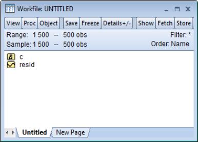
To structure an existing workfile, select in the main workfile window, or double-click on the portion of the window displaying the current range (“Range:”).
Selecting a Workfile Type
EViews opens the dialog. The basic structure of the dialog is quite similar to the dialog (
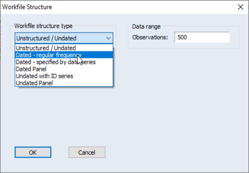
“Creating a Workfile”). On the left-hand side is a dropdown menu where you will select a structure type.
Clicking on the structure type dropdown menu brings up several choices. As before, you may choose between the , and types. There are, however, several new options. In the place of , you have the option to select from , , , or .
Workfile Structure Settings
As you select different workfile structure types, the right-hand side of the dialog changes to show relevant settings and options for the selected type. For example, if you select the , you will be prompted to enter information about the frequency of your data and date information; if you select an , you will be prompted for information about identifiers and the handling of balancing operations.
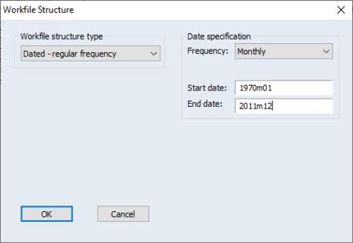
Dated - Regular Frequency
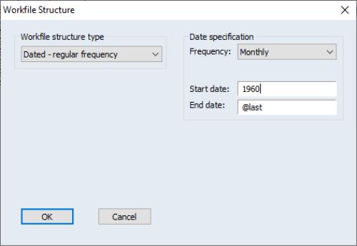
Given an existing workfile, the simplest method for defining a regular frequency structured workfile is to select in the structure type dropdown menu. The right side of the dialog changes to reflect your choice, prompting you to describe your data structure.
You are given the choice of a , as well as a and . The only difference between this dialog and the workfile create version is that the field is pre-filled with “@LAST”. This default reflects the fact that given a start date and the number of observations in the existing workfile, EViews can calculate the end date implied by “@LAST”. Alternatively, if we provide an ending date, and enter “@FIRST” in the field, EViews will automatically calculate the date associated with “@FIRST”.
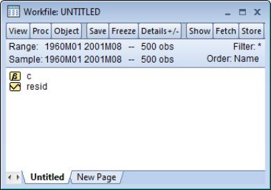
If we fill out the desired fields and click on , EViews will restructure the workfile. In this example, we have specified a monthly frequency starting in 1960m01 and continuing until “@LAST”. There are exactly 500 observations in the workfile since the end date was calculated to match the existing workfile size.
Alternatively, we might elect to enter explicit values for both the starting and ending dates. In this case, EViews will calculate the number of observations implied by these dates and the specified frequency. If the number does not match the number of observations in the existing workfile, you will be informed of this fact, and prompted to continue. If you choose to proceed, EViews will both restructure and resize the workfile to match your specification.
One consequence of this behavior is that resizing a workfile is a particular form of restructuring. To resize a workfile, simply call up the dialog, and change the beginning or ending date.
Here we have changed the from “2011m08” to “2011m12”, thereby instructing EViews to add 4 observations to the end of the workfile. If you select , EViews will inform you that it will add 4 observations and prompt you to continue. If you proceed, EViews will resize the workfile to your specification.
Specifying Start and End Times
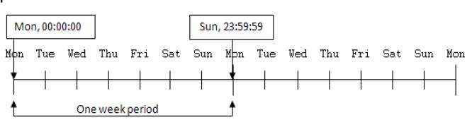
The method used to specify the start and end dates or times should be discussed a bit further. Time periods are generally specified by intervals, such that an hour is represented by the specification 00:00 to 59:59. Thus, a full 24 hour day is defined with a start time of 00:00:00 and an end time of 23:59:59. You will notice that for intraday data, the defaults provided by EViews when you create a workfile reflect this. Similarly, a seven day week can be defined from Monday at 00:00:00 through Sunday at 23:59:59. One second after this ending time, 24:00:00, refers to the following Monday at midnight and is the first second of the next period.
Not only does specifying an end time of 24:00:00 extend into the next day by one second, it will extend by an amount relative to the frequency being defined for the workfile. For instance, given an hourly workfile, an end time of 24:00:00 would add an extra hour to each day, since extending even a second into the next period adds a full interval.
In general, when specifying a range of time for observations, time can be looked at in terms of intervals or in terms of single measurements. For example, the time period 9 a.m. to 12 p.m. can be considered to be three hourly intervals: 9 a.m. to 10 a.m., 10 a.m. to 11 a.m, and 11 a.m. to 12 p.m. Alternately, it could be considered as four on-the-hour measurements: the first at 9 a.m., the second at 10 a.m., the third at 11 a.m., and the fourth at 12 p.m. While the interval model may be more frequently used for continuous measurements over time, it is really up to you to decide which model fits your data better.
In the first case, which defines three intervals from 9 a.m. to 12 p.m., you would specify your workfile with a start time of 9 a.m. and an end time of 11 a.m. This may not seem intuitive, but remember that specifying an end time of 12 p.m. would add an additional hour, defining the interval from 12 p.m. to 1 p.m. In fact, you could specify any end time from 11:00:00 to 11:59:59 for the third interval.
If we wish to look at our data in terms of four discrete hourly measurements, as in the second case, we would specify our workfile with a start time of 9 a.m. and an end time of 12 p.m. Our data points could then be measured at 9 a.m., 10 a.m., 11 a.m., and 12 p.m.
The distinction between thinking of time in terms of intervals or as discrete measurements is subtle. Generally, simply remember that the starting time will be defined as the first observation, and the following observations are defined by the length of time between the starting time and each subsequent time period. Specifying a start time of 9 a.m. and an end time of 9 a.m. will generate a workfile with one observation per day. To determine the number of observations, subtract the start time from the end time and add one for the first observation.
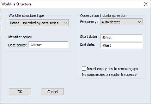
Dated - specified by date series
The second approach to structuring your workfile is to provide the name of a series containing the dates (or series than may be interpreted as dates) to be used as observation identifiers. Select in the dropdown menu, and fill out the remainder of the dialog.
The first thing you must do is enter the name of one or more that describe the unique date identifiers.
The series may contain EViews date values (a true date series), or the single or multiple series may contain numeric or string representations of unique dates. In the latter case, EViews will create a single date series containing the date values associated with the numeric or string representations. This new series, which will be given a name of the form DATEID##, will be used as the identifier series.
On the right side of the dialog, you will specify additional information about your workfile structure. In the first dropdown menu, you will choose one of the standard EViews workfile frequencies (annual, quarterly, monthly, etc.). As shown in the image, there is an additional (default) option, , where EViews attempts to detect the frequency of your data from the values in the specified series. In most cases you should use the default; if, however, you choose to override the auto-detection, EViews will associate the date values in the series with observations in the specified frequency.
You may elect to use the EViews defaults, “@FIRST” and “@LAST”, for the and the . In this case, the earliest and latest dates found in the identifier series will be used to define the observations in the workfile. Alternatively, you may specify the start and end dates explicitly. If these dates involve resizing the workfile, you will be informed of this fact, and prompted to continue.
The last option is the checkbox. This option should be used if you wish to ensure that you have a regular frequency workfile. If this option is selected, EViews will add any observations necessary to remove gaps in the calendar at the given frequency. If the option is not selected, EViews will use only the observed IDs in the workfile and the workfile may be structured as an irregular workfile.
Suppose, for example, that you have observation with IDs for the quarters 1990Q1, 1990Q2, 1990Q4, but not 1990Q3. If is checked, EViews will remove the gap in the calendar by adding an observation corresponding to 1990:3. The resulting workfile will be structured as a regular quarterly frequency workfile. If you do not insert observations, the workfile will be treated as an irregular quarterly workfile.
Once you click on , EViews will first look for duplicate observation IDs. If duplicates are not found, EViews will sort the data in your workfile by the values in the date series and define the specified workfile structure. In addition, the date series is locked so that it may not be altered, renamed, or deleted so long as it is being used to structure the workfile.
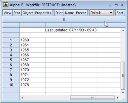
To illustrate the process of structuring a workfile by an ID series, we consider a simple example involving a 10 observation unstructured workfile.
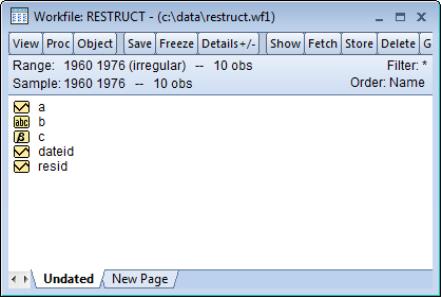
Suppose that the workfile contains the alpha series B consisting of string representations of dates, as depicted. The first thing you should notice about B is that the years are neither complete, nor ordered—there is, for example, no “1962,” and “1965” precedes “1961”. You should also note that since we have an unstructured workfile, the observation identifiers used to identify the rows of the table are given by the default integer values.
From the workfile window we call up the dialog, select as our workfile type, and enter the name “B” in the edit box. We will start by leaving all of the other settings at their defaults: the frequency is set at , and the start and end dates are given by “@FIRST” and “@LAST”.
The resulting (structured) workfile window shown here indicates that we have a 10 observation irregular annual frequency workfile that ranges from an earliest date of 1960 to the latest date of 1976
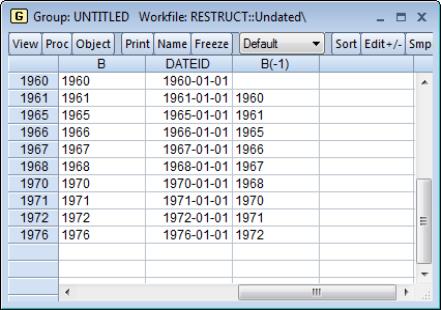
Since the series B contained only text representations of dates, EViews has created a new series DATEID containing date values corresponding to those in B. DATEID is locked and cannot be altered, renamed, or deleted so long as it is used to structure the workfile.
Here, we show a group containing the original series B, the new series DATEID, and the lag of B, B(-1). There are a few things to note. First, the observation identifiers are no longer integers, but instead are values taken from the identifier series DATEID. The formatting of the observation labels will use the display formatting present in the ID series. If you wish to change the appearance of the labels, you should set the display format for DATEID (see
“Display Formats”).
Second, since we have sorted the contents of the workfile by the ID series, the values in B and DATEID are ordered by date. Third, the lagged values of series use the irregular calendar defined by DATEID—for example, the lag of the 1965 value is given by 1961.
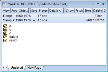
Alternately, we could have chosen to restructure with the checkbox selected, thus ensuring that we have a regular frequency workfile.
To see the effect of this option, we may reopen the dialog by double clicking on the “Range:” string near the top of the workfile window, selecting the option, and then clicking on . EViews will inform us that the restructure option involves creating 7 additional observations, and will prompt us to continue. Click on again to proceed. The workfile will be converted to a regular frequency annual workfile with observations from 1960 to 1976.
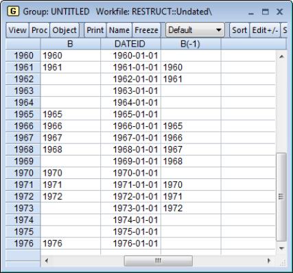
We again show the group containing B, DATEID, and B(-1). Notice that while the observation identifiers and DATEID now include values for the previously missing dates, B and B(-1), do not. When EViews adds observations in the restructure operation, it sets all ordinary series values to NA or missing for those new observations. You are responsible for filling in values as desired.
Dated Panels
To create a dated panel workfile, you should call up the dialog then select as our structure type.
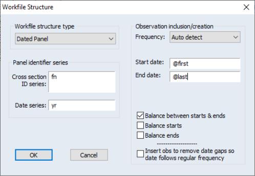
There are three parts to the specification of a dated panel. First, you must specify one or more that describe date identifiers that are unique within each group. Next, you must specify the that identify members of a given group. Lastly, you should set options which govern the choice of frequency of your dated data, starting and ending dates, and the adding of observations for balancing the panel or ensuring a regular frequency.
Dated Panel Basics
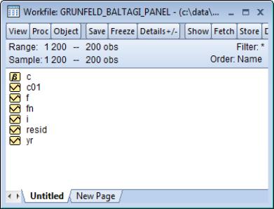
We begin by considering the Grunfeld data that have been described in a number of places (see, for example, Baltagi (2005), Econometric Analysis of Panel Data, Third Edition, from which this version of the data has been taken). The data measure R&D expenditure and other economic measures for 10 firms for the years 1935 to 1954. These 200 observations form a balanced panel dataset. We begin by reading the data into an unstructured, 200 observation workfile.
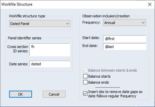
To structure the panel for these data, we call up the dialog, select as our structure type, and enter the name of the representing firm number, FN, along with the (cell ID) representing the year, YR. If we leave the remaining settings at their default values, EViews will auto detect the frequency of the panel, setting the start and end dates on the basis of the values in the YR series, and will add any observations necessary so that the data between the starts and ends is balanced.
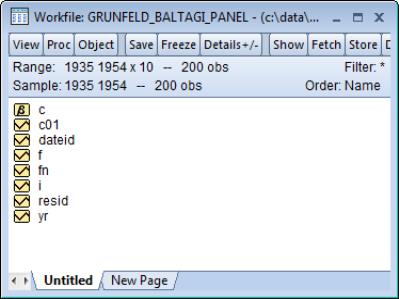
When you click on to accept these settings, EViews creates a DATEID series, sorts the data by ID and DATEID, locks the two series, and applies the structure. The auto detecting of the date frequency and endpoints yields an annual (balanced) panel beginning in 1935 and ending in 1954.
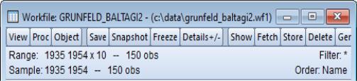
The basic information about this structure is displayed at the top of the workfile window. There are a total of 200 observations representing a balanced panel of 10 cross-sections with data from 1935 to 1954.
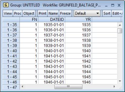
Notice that the observation labels for the structured panel workfile show both the group identifier and the cell identifier.
Dated Panel Balancing
In the basic Grunfeld example, the data originally formed a balanced panel so the various balance operations have no effect on the resulting workfile. Similarly, the option to insert observations to remove gaps has no effect since the data already follow a regular (annual) frequency with no gaps.
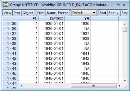
Let us now consider a slightly more complicated example involving panel data that are both unbalanced and irregular. For simplicity, we have created an unbalanced dataset by taking a 150 observation subset of the 200 observations in the Grunfeld dataset.
First, we call up the dialog and again select . We begin by using FN and YR as our group and cell IDs, respectively. Use to determine the frequency, do not perform any balancing, and click on . With these settings, our workfile will be structured as an unbalanced, irregular, annual workfile ranging from 1935 to 1954.
Alternatively, we can elect to perform one or more forms of balancing either at the time the panel structure is put into place, or in a restructure step. Simply call up the dialog and select the desired forms of balancing. If you have previously structured your workfile, the dialog will be pre-filled with the existing identifiers and frequency. In this example, we will have our existing annual panel structure with identifiers DATEID and FN.
In addition to choosing whether to and , you may choose, at most, one of the two options , and .
If balancing between starts and ends, the balancing procedure will use the observed cell IDs (in this case, the years encoded in DATEID for all cross-sections) between a given start and end date. All cross-sections will share the same possibly irregular calendar for observations between their starts and ends. If you also elect to insert observations to remove date gaps, EViews balances each cross-section between starts and ends using every date in the calendar for the given frequency. In the latter case, all cross-sections share the same regular calendar for observations between their starts and ends.
Selecting all three options, , and ensures a balanced panel workfile. If we substitute the option for , we further guarantee that the data follow a regular frequency.
In partly or fully balancing the panel workfile, EViews will add observations as necessary, and update the corresponding data in the identifier series. All other variables will have their values for these observations set to NA. Here, we see that EViews has added data for the two identifier series FN and DATEID while the ordinary series YR values associated with the added observations are missing.
Undated with ID series
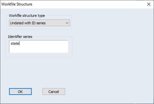
If you wish to provide cross-section identifiers for your undated data, select in the dropdown menu.
EViews will prompt you to enter the names of one or more ID series. When you click on , EViews will first sort the workfile by the values of the ID series, and then lock the series so that it may not be altered so long as the structure is in place. The values of the ID series will now be used in place of the default integer identifiers.
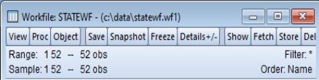
Let us consider a simple example. Suppose that we have a 52 observation unstructured workfile, with observations representing the 50 states in the U.S., D.C., and Puerto Rico.
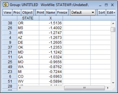
We wish to use the values in the alpha series STATE (which contains the standard U.S. Postal Service abbreviations) to identify the observations. The data for STATE and a second series, X, are displayed here. Notice that the data are ordered from low to high values for X.
Simply select , enter “state” as the identifier series, and click to accept the settings. EViews will sort the observations in the workfile by the values in the ID series, and then apply the requested structure, using and locking down the contents of STATE.
Visually, the workfile window will change slightly with the addition of the description “(indexed)” to the upper portion of the window, showing that the workfile has been structured. Note, however, that since the dataset is still undated, the workfile range and sample are still expressed in integers (“1 52”).
To see the two primary effects of structuring cross-section workfiles, we again examine the values of STATE and the variable X. Notice that the data have been sorted (in ascending order) by the value of STATE and that the observation identifiers in the left-hand border now use the values of STATE.
Note that as with irregular structured workfiles, the observation labels will adopt the characteristics of the classifier series display format. If you wish to change the appearance of the observation labels, you should set the spreadsheet display format for STATE (see
“Changing the Spreadsheet Display”).
Undated Panels
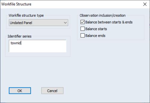
To apply an undated panel structure to your workfile, you must specify one or more that identify members of a given group. First, select from the dropdown menu, and then enter the names of your . You may optionally instruct EViews to balance between the starts and ends, the starts, or the ends of your data.
As an example, we consider the Harrison and Rubinfeld data on house prices for 506 observations located in 92 towns and cities in the harbor area near New Bedford, MA (Harrison and Rubinfeld 1978; Gilley and Pace 1996).
The group identifiers for these data are given by the series TOWNID, in which the town for a given observation is coded from 1 to 92. Observations within a town are not further identified, so there is no cell ID within the data. Here we specify only the group identifier TOWNID.
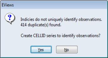
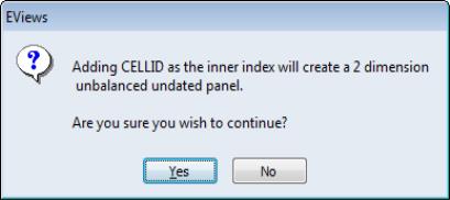
When we click on , EViews analyzes the data in TOWNID and determines that there are duplicate observations—there are, for example, 22 observations with a TOWNID of 5. Since TOWNID does not uniquely identify the individual observations, EViews prompts you to create a new cell ID series.
If you click on , EViews will return you to the specification page where you may define a different set of group identifiers. If you choose to continue, EViews will create a new series with a name of the form CELLID## (e.g., CELLID, CELLID01, CELLID02, etc.) containing the default integer cell identifiers. This series will automatically be used in defining the workfile structure.
There are important differences between the two approaches (
i.e., creating a new ID series, or providing a second ID series in the dialog) that are discussed in
“Lags, Leads, and Panel Structured Data”. In most circumstances, however, you will click on to continue. At this point, EViews will inform you that you have chosen to define a two-dimensional, undated panel, and will prompt you to continue. In this example, the data are unbalanced, which is also noted in the prompt.
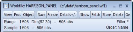
When you click on to continue, EViews will restructure the workfile using the identifiers TOWNID and CELLID##. The data will be sorted by the two identifiers, and the two-dimensional panel structure applied. The workfile window will change to show this restructuring. As depicted in the upper portion, we have a 506 observation, undated panel with dimension (92, 30)—92 groups with a maximum of 30 observations in any group.
Note that in this example, balancing the starts or interiors has no effect on the workfile since CELLID## has cell IDs that begin at 1 and run consecutively for every group. If, however, we choose to balance the ends, which vary between 1 and 30, the corresponding resize operation would add 2254 observations. The final result would be a workfile with 2760 observations, comprised of 92 groups, each with 30 observations.
Common Structuring Errors
In most settings, you should find that the process of structuring your workfile is relatively straightforward. It is possible, however, to provide EViews with identifier information that contains errors so that it is inconsistent with the desired workfile structure. In these cases, EViews will either error, or issue a warning and offer a possible solution. Some common errors warrant additional discussion.
Non-unique identifiers
The most important characteristic of observation identifiers is that they uniquely identify every observation. If you attempt to structure a workfile with identifiers that are not unique, EViews will warn you of this fact, will offer to create a new cell ID, and will prompt you to proceed. If you choose to proceed, EViews will then prompt you to create a panel workfile structure using both the originally specified ID(s) and the new cell ID to identify the observations. We have seen an example of this behavior in our discussion of the undated panel workfile type (
“Undated Panels”).
In some cases, however, this behavior is not desired. If EViews reports that your date IDs are not unique, you might choose to go back and either modify or correct the original ID values, or specify an alternate frequency in which the identifiers are unique. For example, the date string identifier values “1/1/2002” and “2/1/2002” are not unique in a quarterly workfile, but are unique in a monthly workfile.
Invalid date identifiers
When defining dated workfile structures, EViews requires that you enter the name or names of series containing date information. This date information may be in the form of valid EViews date values, or it may be provided in numbers or strings which EViews will attempt to interpret as valid date values. In the latter case, EViews will attempt to create a new series containing the interpreted date values.
If EViews is unable to translate your date information into date values, it will issue an error indicating that the date series has invalid values or that it is unable to interpret your date specification. You must either edit your date series, or structure your workfile as an undated workfile with an ID series.
In cases where your date information is valid, but contains values that correspond to unlikely dates, EViews will inform you of this fact and prompt you to continue. Suppose, for example, that you have a series that contains 4-digit year identifiers (“1981,” “1982,” etc.), but also has one value that is coded as a 2-digit year (“80”). If you attempt to use this series as your date series, EViews will warn you that it appears to be an integer series and will ask you if you wish to recode the data as integer dates. If your proceed, EViews will alter the values in your series and create an integer dated (i.e., not time dated) workfile, which may not be what you anticipated.
Alternately, you may cancel the restructure procedure, edit your date info series so that it contains valid values, and reattempt to apply a structure.
Missing value identifiers
Your identifier series may be numeric or alpha series containing missing values. How EViews handles these missing values depends on whether the series is used as a date ID series, or as an observation or group ID series.
Missing values are not allowed in situations where EViews expects date information. If EViews encounters missing values in a date ID series, it will issue a warning and will prompt you to delete the corresponding observations. If you proceed, EViews will remove the observations from the workfile. If removed, the observations may not be recovered, even if you subsequently change or remove the workfile structure.
If the missing values are observed in an observation or group ID series, EViews will offer you a choice of whether to keep or remove the corresponding observations, or whether to cancel the restructure. If you choose to keep the observations, the missing value, NA, for numeric series, and a blank string for alpha series, will be used as an observation or cross-section ID in the restructured workfile. If you choose to drop the observations, EViews will simply remove them from the workfile. These observations may not be recovered.
Removing a Workfile Structure
You may remove a workfile structure at any time by restructuring to an unstructured or regular frequency dated workfile. Call up the dialog and select or from the dropdown menu. Fill out the appropriate entries and click .
EViews will remove the workfile structure and will unlock any series used as date, group, or observation identifiers.