Census X-13 in EViews 8

EViews 8 offers an easy-to-use front-end for working with the U.S. Census Bureau’s X-13 seasonal adjustment tools. In addition to providing a wide range of new features, X-13 is capable of performing updated versions of X-11/X-12 or TRAMO/SEATS ARIMA seasonal adjustment.

Although the EViews interface supports the majority of options available in X-13, not all are supported. However missing options can be implemented via the EViews command line, or by providing your own X-13 specification files. The EViews interface lets you save the X-13 specification file it generates so that you may customize it for future analysis.

X-13 Example

As an example of using the EViews X-13 proc, we will seasonally adjust monthly employment data obtained from the Federal Reserve Economic Data (FRED) database. The EViews workfile, X13 Macro.wf1, contains monthly non-seasonally adjusted US unemployment data from January 2005 to June 2012 in a series called UNRATENSA. We will perform two types of seasonally adjustment: X-11 with automatic ARIMA selection performed using X-11- Auto, and SEATS based with automatic ARIMA selection performed using TRAMO.

View a video of this Census X-13 example.

To perform X-11 based seasonal adjustment with automatic ARIMA selection using X-11- Auto, open the UNRATENSA series and click on Proc/Seasonal Adjustment/Census X-13. EViews will display the X-13 dialog:

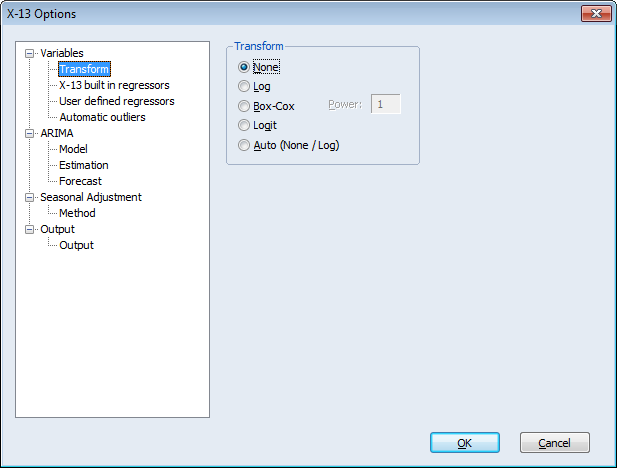
Note that this example will not be using any exogenous variables, transformations or outliers in the model so skip the settings in the Variables branch of the tree structure.

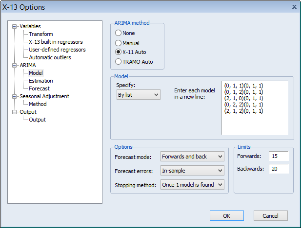
Click on the ARIMA branch to display the ARIMA options. Select X-11 Auto as the ARIMA Method, and leave the remaining options at their default values:

Open the Seasonal Adjustment branch and select X-11 as the Seasonal adjustment method

Select the Output branch and check all four of the Final series output boxes so that EViews will import the seasonally adjusted values, the trend values (D12), the seasonal factors (D10) and the irregular components (D13) into the workfile.

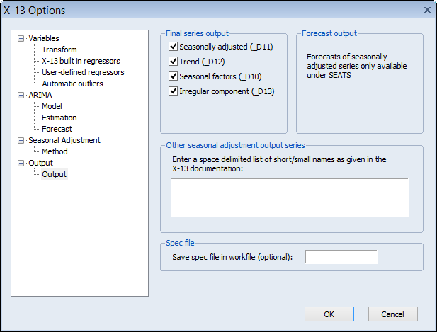
After you click on OK, EViews will run the X-13ARIMA-SEATS program using the specified settings and will display the text output produced by the program in the series window. In addition, EViews will save the four output series UNRATENSA_D10, UNRATENSA_D11, UNRATENSA_D12 and UNRATENSA_D13 in the workfile.

UNRATENSA_D11 contains the final seasonally adjusted series. Select this series along with the original UNRATENSA, right-click and Open/As group, then select View/Graph and click on OK to display a line graph of the adjusted and unadjusted series:

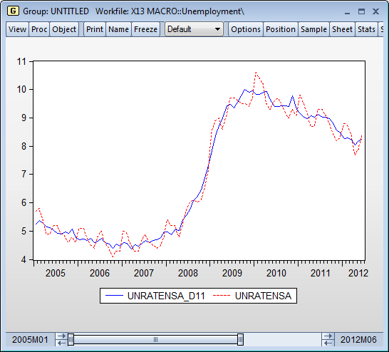
The smoothed series UNRATENSA_D11 clearly exhibits less seasonally volatility than the original series UNRATENSA.

Displaying the graph views of the remaining series lets you view the individual components of the smoothing. For example, showing a graph of UNRATENSA_D12 enables you to see the trend component.

For comparison purposes, we perform SEATS based seasonal adjustment with automatic outlier detection on the same data. Select Proc/Seasonal Adjustment/ Census X-13 from the series menu to display the X-13 dialog, then open the Variables branch of the dialog and click on the Automatic outliers node. Instruct EViews to perform automatic outlier selection by checking all four of the Outlier types boxes (Additive, Level shift, Temporary change, Seasonal). Leave the remaining settings at their defaults:

Open the ARIMA branch of the tree, select the Model node, and select TRAMO Auto as the ARIMA Method. Leave all other options at their defaults:

Open the Seasonal Adjustment branch, select SEATS as the Seasonal adjustment method, and select the Append forecasts option:

Finally, switch to the Output branch, select the first four Final series output boxes to instruct EViews to import the seasonally adjusted values, the trend values, the seasonal factors, and the irregular components into the workfile. Note that by default the forecasted seasonal adjustment values (AFD) is selected in the Forecast output box:

Click on OK to run X-13 with these settings and bring the five output series from X- 13 to our workfile. Note that EViews will save the results in the new series UNRATENSA_S10, UNRATENSA_S11, UNRATENSA_S12 and UNRATENSA_S13, and UNRATENSA_AFD.

We may open up a group object containing the seasonally adjusted series, UNRATENSA_S11, along the X-11 seasonally adjusted series UNRATENSA_D11 by selecting the three series, right-clicking and selecting Open/As Group. Extend the workfile sample by two years (24 months) by issuing the command

smpl @first 2012m06+24

select View/Graph and click on OK to display a line graph of the two adjusted and one unadjusted series:

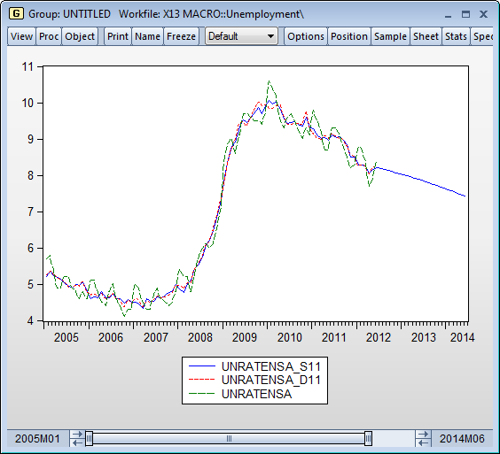
Notice that the SEATS seasonally adjusted series, UNEMPNSA_S11, closely tracks the X- 11 adjusted series, UNEMPNSA_D11, with both offering a seasonally smoother version of the original series.

Also note that since we used the Append forecasts to instruct SEATS to append two years of forecasts to the final seasonally adjusted value, the UNEMPSNA_S11 series continues until June 2014.