Estimating an Equation in EViews
Estimation Methods
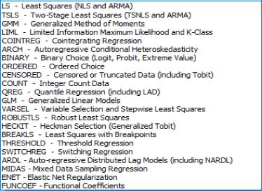
Having specified your equation, you now need to choose an estimation method. Click on the Method: entry in the dialog and you will see a drop-down menu listing estimation methods.
Standard, single-equation regression is performed using least squares. The other methods are described in subsequent chapters.
Equations estimated by cointegrating regression, GLM or stepwise, or equations including MA terms, may only be specified by list and may not be specified by expression. All other types of equations (among others, ordinary least squares and two-stage least squares, equations with AR terms, GMM, and ARCH equations) may be specified either by list or expression. Note that some equations, such as quantile regression may be specified by expression, but only linear specifications are permitted.
Estimation Sample
You should also specify the sample to be used in estimation. EViews will fill out the dialog with the current workfile sample, but you can change the sample for purposes of estimation by entering your sample string or object in the edit box (see
“Samples” for details). Changing the estimation sample does not affect the current workfile sample.
If any of the series used in estimation contain missing data, EViews will temporarily adjust the estimation sample of observations to exclude those observations (listwise exclusion). EViews notifies you that it has adjusted the sample by reporting the actual sample used in the estimation results:
Here we see the top of an equation output view. EViews reports that it has adjusted the sample. Out of the 372 observations in the period 1959M01–1989M12, EViews uses the 340 observations with valid data for all of the relevant variables.
You should be aware that if you include lagged variables in a regression, the degree of sample adjustment will differ depending on whether data for the pre-sample period are available or not. For example, suppose you have nonmissing data for the two series M1 and IP over the period 1959M01–1989M12 and specify the regression as:
m1 c ip ip(-1) ip(-2) ip(-3)
If you set the estimation sample to the period 1959M01–1989M12, EViews adjusts the sample to:
since data for IP(–3) are not available until 1959M04. However, if you set the estimation sample to the period 1960M01–1989M12, EViews will not make any adjustment to the sample since all values of IP(-3) are available during the estimation sample.
Some operations, most notably estimation with MA terms and ARCH, do not allow missing observations in the middle of the sample. When executing these procedures, an error message is displayed and execution is halted if an NA is encountered in the middle of the sample. EViews handles missing data at the very start or the very end of the sample range by adjusting the sample endpoints and proceeding with the estimation procedure.
Estimation Options
EViews provides a number of estimation options. These options allow you to weight the estimating equation, to compute heteroskedasticity and auto-correlation robust covariances, and to control various features of your estimation algorithm. These options are discussed in detail in
“Estimation Options”.