Cross-sectionally Independent Panel Unit Root Testing
The unit root test is a cornerstone of modern time series analysis. Nevertheless, a well-known drawback of many popular univariate unit root tests is a lack of statistical power in the presence of small to medium sized samples.
Since many economic time series have short samples but are observed over many cross-sections, multivariate unit root tests that combine results for different cross-sections or series, offer improved statistical power over their univariate counterparts. While these tests are commonly termed “panel unit root” tests, theoretically, they are simply multiple-series unit root tests that have been applied to panel data structures (where the presence of cross-sections generates “multiple series” out of a single series)
EViews computes five different independent cross-section panel unit root tests: Levin, Lin and Chu (2002), Breitung (2000), Im, Pesaran and Shin (2003), Fisher-type tests using ADF and PP tests (Maddala and Wu (1999) and Choi (2001)), and Hadri (2000). Notably all of these tests require cross-sectional independence. Tests which relax this assumption are described in
“Cross-sectionally Dependent Panel Unit Root Tests”.
Bear in mind that while these tests are commonly termed “panel unit root” tests, theoretically, they are simply multiple-series unit root tests that have been applied to panel data structures (where the presence of cross-sections generates “multiple series” out of a single series). Accordingly, EViews supports these tests in settings involving multiple series: as a series view (if the workfile is panel structured), as a group view, or as a pool view.
Performing Independent Panel Unit Root Tests in EViews
The following discussion assumes that you are familiar with the basics of both unit root tests and panel unit root tests. Additional background is provided in
“Independent Panel Unit Root Tests Background”.
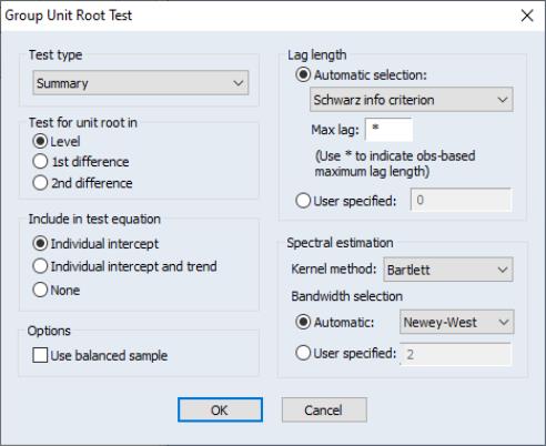
To begin, select from the menu of an EViews group or pool object, or from the menu of an individual series in a panel structured workfile. Here we show the dialog for a Group unit root test—the other dialogs differ slightly (for testing using a pool object, there is an additional field in the upper-left hand portion of the dialog where you must indicate the name of the pool series on which you wish to conduct your test; for the series object in a panel workfile, the option is not present).
If you wish to accept the default settings, simply click on OK. EViews will use the default setting, and will compute a full suite of unit root tests on the levels of the series, along with a summary of the results.
To customize the unit root calculations, you will choose from a variety of options. The options on the left-hand side of the dialog determine the basic structure of the test or tests, while the options on the right-hand side of the dialog control advanced computational details such as bandwidth or lag selection methods, or kernel methods.
The dropdown menu at the top of the dialog is where you will choose the type of test to perform. There are six settings: “ “”, “”, “, “, “, and “, corresponding to one or more of the tests listed above. The dropdown menu labels include a brief description of the assumptions under which the tests are computed. “Common root” indicates that the tests are estimated assuming a common AR structure for all of the series; “Individual root” is used for tests which allow for different AR coefficients in each series.
We have already pointed out that the default instructs EViews to estimate the first five of the tests, where applicable, and to provide a brief summary of the results. Selecting an individual test type allows you better control over the computational method and provides additional detail on the test results.
The next two sets of radio buttons allow you to control the specification of your test equation. First, you may choose to conduct the unit root on the , , or of your series. Next, you may choose between sets of exogenous regressors to be included. You can select if you wish to include individual fixed effects, to include both fixed effects and trends, or for no regressors.
The option is present only if you are estimating a Pool or a Group unit root test. If you select this option, EViews will adjust your sample so that only observations where all series values are not missing will be included in the test equations.
Depending on the form of the test or tests to be computed, you will be presented with various advanced options on the right side of the dialog. For tests that involve regressions on lagged difference terms (Levin, Lin, and Chu, Breitung, Im, Pesaran, and Shin, Fisher - ADF) these options relate to the choice of the number of lags to be included. For the tests involving kernel weighting (Levin, Lin, and Chu, Fisher - PP, Hadri), the options relate to the choice of bandwidth and kernel type.
For a group or pool unit root test, the EViews default is to use automatic selection methods: information matrix criterion based for the number of lag difference terms (with automatic selection of the maximum lag to evaluate), and the Andrews or Newey-West method for bandwidth selection. For unit root tests on a series in a panel workfile, the default behavior uses user-specified options.
If you wish to override these settings, simply enter the appropriate information. You may, for example, select a fixed, user-specified number of lags by entering a number in the field. Alternatively, you may customize the settings for automatic lag selection method. Alternative criteria for evaluating the optimal lag length may be selected via the dropdown menu (Akaike, Schwarz, Hannan-Quinn, Modified Akaike, Modified Schwarz, Modified Hannan-Quinn), and you may limit the number of lags to try in automatic selection by entering a number in the box. For the kernel based methods, you may select a kernel type from the dropdown menu (, , ), and you may specify either an automatic bandwidth selection method (, ) or user-specified fixed bandwidth.
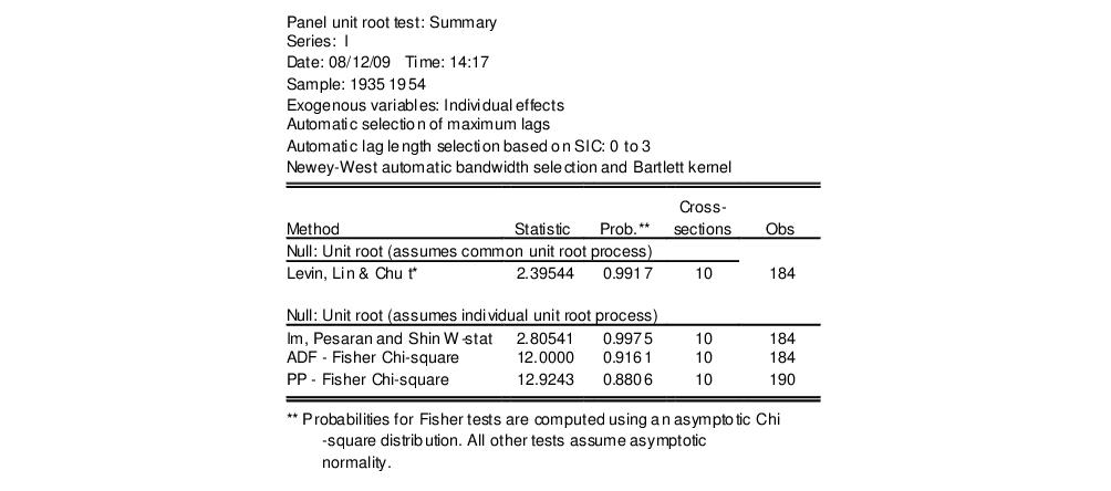
As an illustration, we perform a panel unit root tests on real gross investment data (I) in the oft-cited Grunfeld data containing data on R&D expenditure and other economic measures for 10 firms for the years 1935 to 1954 found in “Grunfeld_Baltagi_Panel.WF1”. We compute the summary panel unit root test, using individual fixed effects as regressors, and automatic lag difference term and bandwidth selection (using the Schwarz criterion for the lag differences, and the Newey-West method and the Bartlett kernel for the bandwidth). The results for the panel unit root test are presented below:
The top of the output indicates the type of test, exogenous variables and test equation options. If we were instead estimating a Pool or Group test, a list of the series used in the test would also be depicted. The lower part of the summary output gives the main test results, organized both by null hypothesis as well as the maintained hypothesis concerning the type of unit root process.
All of the results indicate the presence of a unit root, as the LLC, IPS, and both Fisher tests fail to reject the null of a unit root.
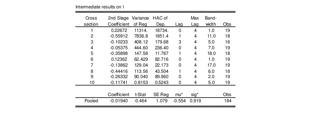
If you only wish to compute a single unit root test type, or if you wish to examine the tests results in greater detail, you may simply repeat the unit root test after selecting the desired test in dropdown menu. Here, we show the bottom portion of the LLC test specific output for the same data:
For each cross-section, the autoregression coefficient, variance of the regression, HAC of the dependent variable, the selected lag order, maximum lag, bandwidth truncation parameter, and the number of observations used are displayed.
Independent Panel Unit Root Tests Background
Panel unit root tests are similar, but not identical, to unit root tests carried out on a single series. Here, we briefly describe the five panel unit root tests currently supported in EViews; for additional detail, we encourage you to consult the original literature. The discussion assumes that you have a basic knowledge of unit root theory.
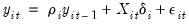
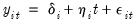
We begin by classifying our unit root tests on the basis of whether there are restrictions on the autoregressive process across cross-sections or series. Consider a following AR(1) process for panel data:
 | (42.63) |
where
cross-section units or series, that are observed over periods
.
The

represent the exogenous variables in the model, including any fixed effects or individual trends,

are the autoregressive coefficients, and the errors

are assumed to be mutually independent idiosyncratic disturbance. If

,

is said to be weakly (trend-) stationary. On the other hand, if

then

contains a unit root.
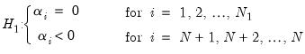
For purposes of testing, there are two natural assumptions that we can make about the

. First, one can assume that the persistence parameters are common across cross-sections so that

for all

. The Levin, Lin, and Chu (LLC), Breitung, and Hadri tests all employ this assumption. Alternatively, one can allow

to vary freely across cross-sections. The Im, Pesaran, and Shin (IPS), and Fisher-ADF and Fisher-PP tests are of this form.
Tests with Common Unit Root Process
Levin, Lin, and Chu (LLC), Breitung, and Hadri tests all assume that there is a common unit root process so that

is identical across cross-sections. The first two tests employ a null hypothesis of a unit root while the Hadri test uses a null of no unit root.
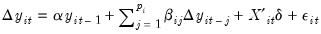
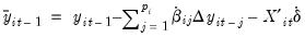
LLC and Breitung both consider the following basic ADF specification:
 | (42.64) |
where we assume a common

, but allow the lag order for the difference terms,

, to vary across cross-sections. The null and alternative hypotheses for the tests may be written as:
 | (42.65) |
 | (42.66) |
Under the null hypothesis, there is a unit root, while under the alternative, there is no unit root.
Levin, Lin, and Chu
The method described in LLC derives estimates of

from proxies for

and

that are standardized and free of autocorrelations and deterministic components.
For a given set of lag orders, we begin by estimating two additional sets of equations, regressing both

, and

on the lag terms

(for

) and the exogenous variables

. The estimated coefficients from these two regressions will be denoted

and

, respectively.
We define

by taking

and removing the autocorrelations and deterministic components using the first set of auxiliary estimates:
 | (42.67) |
Likewise, we may define the analogous

using the second set of coefficients:
 | (42.68) |
Next, we obtain our proxies by standardizing both

and

, dividing by the regression standard error:
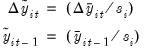 | (42.69) |
where

are the estimated standard errors from estimating each ADF in
Equation (42.64).
Lastly, an estimate of the coefficient

may be obtained from the pooled proxy equation:
 | (42.70) |
LLC show that under the null, a modified
t-statistic for the resulting

is asymptotically normally distributed
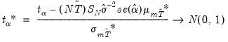 | (42.71) |
where

is the standard
t-statistic for

,

is the estimated variance of the error term

,

is the standard error of

, and:
 | (42.72) |
The remaining terms, which involve complicated moment calculations, are described in greater detail in LLC. The average standard deviation ratio,

, is defined as the mean of the ratios of the long-run standard deviation to the innovation standard deviation for each individual. Its estimate is derived using kernel-based techniques. The remaining two terms,

and

are adjustment terms for the mean and standard deviation.
The LLC method requires a specification of the number of lags used in each cross-section ADF regression,

, as well as kernel choices used in the computation of

. In addition, you must specify the exogenous variables used in the test equations. You may elect to include no exogenous regressors, or to include individual constant terms (fixed effects), or to employ individual constants and trends.
Breitung
The Breitung method differs from LLC in two distinct ways. First, only the autoregressive portion (and not the exogenous components) is removed when constructing the standardized proxies:
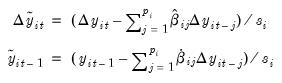 | (42.73) |
where

,

, and

are as defined for LLC.
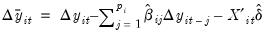
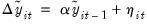
Second, the proxies are transformed and detrended,
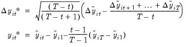 | (42.74) |
The persistence parameter

is estimated from the pooled proxy equation:
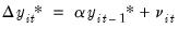 | (42.75) |
Breitung shows that under the null, the resulting estimator

is asymptotically distributed as a standard normal.
The Breitung method requires only a specification of the number of lags used in each cross-section ADF regression,

, and the exogenous regressors. Note that in contrast with LLC, no kernel computations are required.
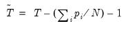
Hadri
The Hadri panel unit root test is similar to the KPSS unit root test, and has a null hypothesis of no unit root in any of the series in the panel. Like the KPSS test, the Hadri test is based on the residuals from the individual OLS regressions of

on a constant, or on a constant and a trend. For example, if we include both the constant and a trend, we derive estimates from:
 | (42.76) |
Given the residuals

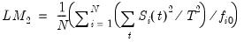
from the individual regressions, we form the LM statistic:
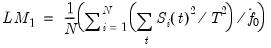 | (42.77) |
where

are the cumulative sums of the residuals,
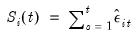 | (42.78) |
and

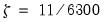
is the average of the individual estimators of the residual spectrum at frequency zero:
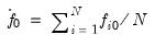 | (42.79) |
EViews provides several methods for estimating the

. See
“Unit Root Testing” for additional details.
An alternative form of the LM statistic allows for heteroskedasticity across

:
 | (42.80) |
Hadri shows that under mild assumptions,
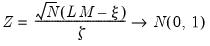 | (42.81) |
where

and

, if the model only includes constants (

is set to 0 for all

), and

and
, otherwise.
The Hadri panel unit root tests require only the specification of the form of the OLS regressions: whether to include only individual specific constant terms, or whether to include both constant and trend terms. EViews reports two

-statistic values, one based on

with the associated homoskedasticity assumption, and the other using

that is heteroskedasticity consistent.
It is worth noting that simulation evidence suggests that in various settings (for example, small

), Hadri's panel unit root test experiences significant size distortion in the presence of autocorrelation when there is no unit root. In particular, the Hadri test appears to over-reject the null of stationarity, and
may yield results that directly contradict those obtained using alternative test statistics (see Hlouskova and Wagner (2006) for discussion and details).
Tests with Individual Unit Root Processes
The Im, Pesaran, and Shin, and the Fisher-ADF and PP tests all allow for individual unit root processes so that

may vary across cross-sections. The tests are all characterized by the combining of individual unit root tests to derive a panel-specific result.
Im, Pesaran, and Shin
Im, Pesaran, and Shin begin by specifying a separate ADF regression for each cross section:
 | (42.82) |
The null hypothesis may be written as,
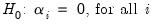 | (42.83) |
while the alternative hypothesis is given by:
 | (42.84) |
(where the

may be reordered as necessary) which may be interpreted as a non-zero fraction of the individual processes is stationary.
After estimating the separate ADF regressions, the average of the
t-statistics for

from the individual ADF regressions,

:
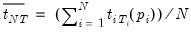 | (42.85) |
is then adjusted to arrive at the desired test statistics.
In the case where the lag order is always zero (

for all

), simulated critical values for

are provided in the IPS paper for different numbers of cross sections

, series lengths

, and for test equations containing either intercepts, or intercepts and linear trends. EViews uses these values, or linearly interpolated values, in evaluating the significance of the test statistics.
In the general case where the lag order in
Equation (42.82) may be non-zero for some cross-sections, IPS show that a properly standardized

has an asymptotic standard normal distribution:
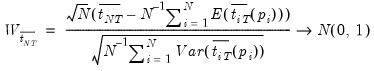 | (42.86) |
The expressions for the expected mean and variance of the ADF regression
t-statistics,

and

, are provided by IPS for various values of

and

and differing test equation assumptions, and are not provided here.
The IPS test statistic requires specification of the number of lags and the specification of the deterministic component for each cross-section ADF equation. You may choose to include individual constants, or to include individual constant and trend terms.
Fisher-ADF and Fisher-PP
An alternative approach to panel unit root tests uses Fisher’s (1932) results to derive tests that combine the p-values from individual unit root tests. This idea has been proposed by Maddala and Wu, and by Choi.
If we define

as the
p-value from any individual unit root test for cross-section

, then under the null of unit root for all

cross-sections, we have the asymptotic result that
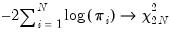 | (42.87) |
In addition, Choi demonstrates that:
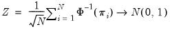 | (42.88) |
where

is the inverse of the standard normal cumulative distribution function.
EViews reports both the asymptotic

and standard normal statistics using ADF and Phillips-Perron individual unit root tests. The null and alternative hypotheses are the same as for the as IPS.
For both Fisher tests, you must specify the exogenous variables for the test equations. You may elect to include no exogenous regressors, to include individual constants (effects), or include individual constant and trend terms.
Additionally, when the Fisher tests are based on ADF test statistics, you must specify the number of lags used in each cross-section ADF regression. For the PP form of the test, you must instead specify a method for estimating

. EViews supports estimators for

based on kernel-based sum-of-covariances. See
“Frequency Zero Spectrum Estimation” for details.