Cross-sectionally Dependent Panel Unit Root Tests
In
“Cross-sectionally Independent Panel Unit Root Testing”, we described first generation panel unit root tests on pooled panel data, with (possibly) individual trend, intercepts, and lag coefficients when there is cross-sectional independence.
The assumption of cross-sectional independence can be difficult to justify, as cross-sections are often influenced by common forces, termed factors. For instance, cross-country purchasing power parity (PPP) data is often anchored to a common numeraire currency such as the US dollar, so that movements in the latter affect the cross-sectional PPP in correlated fashion. Tests which account for cross-sectional dependence have been termed second generation panel unit root tests.
EViews currently supports two important second generation contributions: Bai and Ng’s (2004) Panel Analysis of Nonstationarity in Idiosyncratic and Common Components (PANIC), and Pesaran’s (2007) Cross-sectionally Augmented IPS (CIPS).
As with independent panel unit root tests, EViews supports testing in different settings involving multiple series: as a series view (if the workfile is panel structured), as a group view, or as a pool view.
Performing Dependent Panel Unit Root Tests in EViews
Second generation panel unit root tests may be performed on a single series in a panel workfile or on a group of series in a workfile. To perform the test in the panel setting, you should open the series and then click on In the group setting, open the group and click on the same view entry. EViews will display the dialog:
There is a lot to this dialog so we will examine each section in turn.
Test
The section of the dialog is used to specify the basic test type:
The dropdown lets you choose between the two second generation panel unit root test types: and .
The dropdown offers three choices for the deterministic terms to be included in the specification: , , or .
ADF Lag Selection
The section controls the specification of the ADF test specifications in the PANIC and CIPS tests.
The dropdown offers several options for determining the number of lagged difference terms
to use in the ADF specifications. You may use the dropdown to select between using information criteria (Akaike, Schwarz, Hannan-Quinn, Modified Akaike, Modified, Schwarz, Modified Hannan-Quinn), performing
t-tests of lag difference variable significance, or providing a user-specified fixed value.
For the information criteria and t-test options, you will be prompted for the maximum number of lags to consider; for the user-specified fixed value, you will be prompted to enter the value itself.
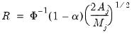
Note that EViews pre-fills the edit field with a default value derived from a variation of the Schwert (1989) rule: let there be a lag choice function
for
and let
; then the default maximum lag
.
PANIC MQ Options
If you choose to perform a PANIC test the section offers options for controlling the computation:
The dropdown lets you choose between the and statistics.
The edit field lets you choose the level of significance at which EViews will perform the test as the p-value for these statistics is obtained by simulation.
The remaining options will change with your selection of the PANIC type:
• If you choose to compute the
, the button will be enabled.
• If you choose
, the will be enabled so that you may control the order of the VAR(
). The settings are as described in
“ADF Lag Selection”.
Factor Selection
The options control the selection of number of factors method used in the PANIC procedure:
The dropdown lets you choose between the , , and . In turn, each of these choices offers different options.
• If you select , you will choose a from the dropdown. You may choose from the following selections: , , .
For the first two selections, the number of factors is determined as the minimum or maximum of the (discussed below), the specified , and of eigenvalues. The will use the average of the other two results.
• If you select , EViews will compute the Bai and Ng (2002) as discussed in
“Bai and Ng”.
The dropdown offers all of the information criteria described by Bai and Ng (, , , , , ) as well as the which averages the criteria prior to determining the optimal number of factors.
• If you select , EViews will compute the Ahn and Horenstein (2013) number of factor determination procedure (
“Ahn and Horenstein”). The dialog looks the same as for , but the dropdown now offers , , and .
• For , the number of factors is specified by the user in the edit box
In all of the automatic factor selection procedures above is the selection of maximum factors to be considered. While ultimately an arbitrary selection, EViews offers some suggestions typically seen in the literature. In particular, as in the case of ADF selection, consider the dropdown which provides the following options:
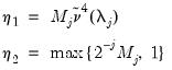
• : let there be a lag choice function
for
and let
; then returns the value
.
• : uses the suggestion made on page 1208 in Ahn and Horenstein (2013).
• : uses
.
• uses

.
• : users can specify an arbitrary value in the edit field.
Furthermore, as discussed in Bai and Ng (2002) and Ahn and Horenstein (2013), factor selection procedures can be improved dramatically if time and/or cross-section dimensions are demeaned and/or standardized. To allow for these possibilities, there are four checkboxes associated with each of these options and combinations:
• : demeans the time dimension.
• : standardizes the time dimension.
• : demeans the cross-section dimension.
• : standardizes the cross-section dimension.
p-value Simulation
In case of the PANIC tests, inference is based on simulated p-values. In this setting, you can may specify simulation options in the p-value section.
In particular, the number of , and can be set in their respective edit fields. Note that the latter is optional. Furthermore, the dropdown offers various random number generators. Details associated with the latter options can be obtained in the EViews documentation for rndseed.
Dependent Panel Unit Root Test Examples
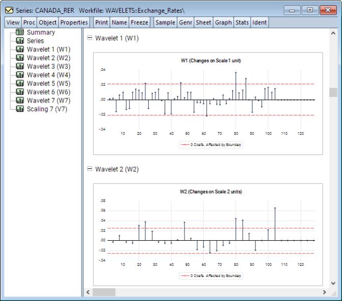
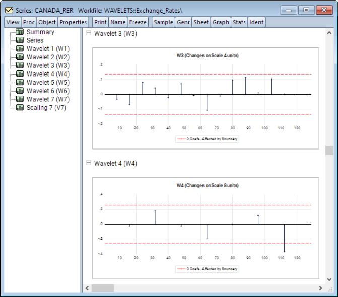
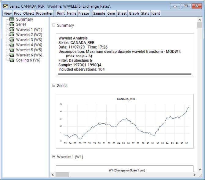
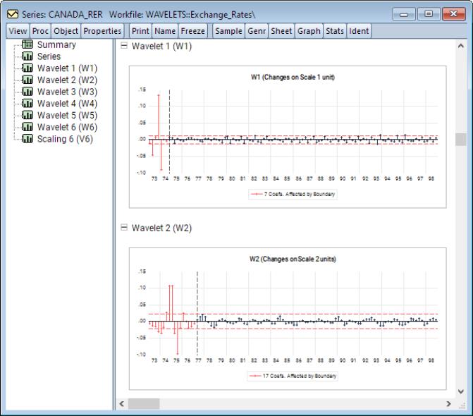
To illustrate some of the features of second generation panel unit root tests in EViews, we consider three examples using data from Pesaran (2007). These panel data feature quarterly real exchange rates from 17 OECD countries for the period 1973q1 to 1998q4. Data can be downloaded from
in the file “real-xrate.zip”.
You may unzip the file then drag-and-drop it onto your EViews to create the new workfile. As is, however, the resulting unstacked, undated workfile is not set up for panel or group unit root testing.
From the command line you can set up the group form of the unstacked data with the following command:
pagestruct(freq=q, start=1973q1)
group oecd_rer *_rate
The first line specifies the frequency of the data (the EViews auto-input was unable to do so since there are no dates in the file). The next line creates a group containing all of the rate series. We can conduct the unit root tests using the group object OECD_RER.
Alternately, we can choose to stack the data in a new page, and conduct the test on the stacked panel data. The command
pagestack ?real_exchange_rate @ ?*
creates a new page containing a stacked panel data series REAL_EXCHANGE_RATE.
Whichever form with which we wish to work, we will use the sample statement
smpl 1974 1998
to the example in Pesaran (2007).
Lastly, note that the examples below use the REAL_EXCHANGE_RATE series in the workfile tab “Realexchangerates7398_STK. All of the examples may also be performed using the group object OECD_RER in the workfile tab “Realexchangerates7398”.
PANIC MQc Example
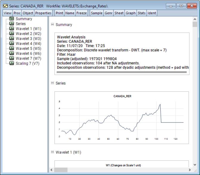
This example will use default values for all inputs. To use the panel data form of the test, click on the workfile tab “Realexchangerates7398_STK”, and then open the panel series REAL_EXCHANGE_RATE. Click on View/Unit Root Tests/Cross-Sectionally Dependent..., to access the second generation panel unit root tests.
As PANIC

is the default test, at this point, one can simply click on to compute this test.
The output displays a spool with the spool tree listing the summary, factor selection, common factors, and individual and pooled idiosyncratic elements. The first of these is a summary of the PANIC procedure performed. The second is a table listing the details of the factor selection procedure. In particular, since the selection was the average of the Bai and Ng (2002) test statistics, listed in the table are the factor selections based on each of the six individual statistic variants as well as their average which is used in the remainder of the PANIC procedure.
Next, the common factors table displays the PANIC test for how many common factors influence the panel. The test statistic and associated p-value are reported. In this particular case, that number selected 7, which is also the maximum number of factors allowed using the Schwert (1989) rule.
The table that follows displays the individual ADF test statistics for the idiosyncratic elements associated with each cross-section. The ADF lags are selected for each cross-section independently using the same automatic selection rule, which in this case happens to be AIC with 7 maximum lags. Furthermore, the columns and report the ADF t-statistic and associated p-value corresponding to the null hypothesis that the idiosyncratic element exhibit a unit root. It is readily seen that apart from Norway, all other cross-sections exhibit a unit root at the 5% significance level.
Lastly, the final table is a pooled version of the individual ADF test statistics in the previous table. Here, we cannot reject the null hypothesis that all of the cross-sections are simultaneously co-integrated.
PANIC MQf Example
For the second example, using the same data, the objective is to perform a PANIC unit root test using the

test statistic and the Ahn and Horenstein (2013) factor selection procedure.
From the series window click on . In the section select in the dropdown. Next, under the group, select from the dropdown. Furthermore, for the , select . Lastly, ensure that , , , and are all checked. Click on .
The spool output display is analogous to that in
“PANIC MQc Example”. Here, the factor selection procedure is based on Ahn and Horenstein (2013).
Evidently, both the eigenvalue ratio and growth ratio statistics select a single common factor using the Ahn and Horenstein (2013) suggestion for maximum factors, which here happens to be 1.
Since the number of common factors selected is 1, the test associated with the common factors is based on an ADF regression. The next table displays the results of this test.
Here, we see that the test fails to reject the null hypothesis that the single common factor is non-stationary.
Next, as in the previous example, table that follows displays the individual ADF test statistics for the idiosyncratic elements associated with each cross-section. Unlike the previous example, there are significantly more cross-sections for which one can argue rejection of the unit root null hypothesis.
Lastly, the pooled version of the latter tests has a p-value which effectively zero, and therefore we fail to reject the null hypothesis that all cross-sections are not cointegrated.
CIPS Example
The final example uses the same data. Here, the objective is to perform the Pesaran (2007) CIPS test. From the series window click on . From the dropdown, select . To conform with the analysis in the original paper, change the dropdown in the group to . We will stick with a single lag for the ADF regression. Hit .
The output displays a spool with the spool tree listing the summary, CIPS and CADF unit root tests, as well as CIPS and CADF critical value interpolations.
The first of the spool tables is a summary of the CIPS procedure performed. The second is a table listing the details of the CIPS test. In particular, the first part of this table displays the critical values for the usual CIPS statistic as well as its truncated version. The second portion of this table summarizes the test results. Note that the t-statistic is displayed along with the associated p-values which are summarized categorically based on the critical values tabulated in Pesaran (2007). Here, we cannot reject the null hypothesis below the 10% significance level. Furthermore, the outcome of this table matches the results reported in Table XI of the original paper.
The next table summarizes the ADF test statistics that are used in the computation of the CIPS statistic.
Here, the first portion of the table summarizes the critical values associated with the CADF statistic as well as its truncated version. The second portion of this table summarizes the test results for each of the cross-sections. In particular, these are t-statistics associated with the cross-sectionally augmented ADF regressions for each of the cross-sections. The table summarizes the t-statistic and p-value category for each of the CADF and truncated CADF test statistics. In particular, here we cannot reject the unit root null hypotheses at significance levels less than 10% for any of the cross-sections.
At last, the remaining two tables summarize the interpolation computation used to derive the critical values reported earlier.
In particular, if the T or N columns display values, it implies that interpolation was done on that dimension of the data.
Dependent Panel Unit Root Tests Background
To formalize the discussion, let
and
, respectively, denote the cross-section and time indices, and consider the following integrated panel data model:
 | (42.89) |
where

is the observed data,

are the model deterministic dynamics, and
are the innovations.
The traditional first generation panel unit root tests of Maddala and Wu (1999), Hadri (2000), Levin, Lin and Chu (2002), and Im, Pesaran and Shin (2003), while differing in unit root parameter heterogeneity assumptions and in test construction approach, all assume that
are independent across
i.
To introduce cross-sectional dependence, we model

as having a factor model structure,
 | (42.90) |
where

is a vector of

common factors generated by a multivariate white noise process

,
 | (42.91) |

denotes a vector of cross-section specific factor loadings, and
is a multivariate idiosyncratic component which is cross-sectionally independent as

is assumed to account for all inter-cross-sectional correlations. When
are not cross-sectionally independent, the factor model governing

is said to be
approximate. As usual,

is the lag operator, and we have the polynomial:
 | (42.92) |
Substituting, an integrated panel model with cross-sectional dependence may be formulated as
 | (42.93) |
Assumptions imposed on

and

govern the nature of the process for
. For example, when

has rank 0,

is non-stochastic and stationary, or

. Alternately, when

has rank

,

is an

process driven by
linearly independent stochastic trends. In particular, when
,

has
common trends and

cointegrated stationary factors.
A crucial feature of these models is that the common factors

and idiosyncratic components

can each be

or

. This generality permits a wide spectrum of possible outcomes for the properties of the observed

. For instance,
is considered

if
either 
or

is

. Alternately, if the number of common trends

,
is deemed conditionally stationary or non-stationary, depending on the properties of the idiosyncratic component

.
For further detail, see Bai and Ng (2004) and Banerjee and Wagner (2009).
PANIC Unit Root Testing
Bai and Ng’s (2004) PANIC (Panel Analysis of Nonstationarity in Idiosyncratic and Common Components) test is widely considered to be the first unit root test for panel data with cross-sectional dependence. The PANIC test is based on a factor model in which non-stationarity can arise from common factors, idiosyncratic components, or both.
The observed series is modeled using
Equation (42.93):
 | (42.94) |
where
 | (42.95) |
and
is a mean zero, stationary, and invertible MA process. PANIC assumes a balanced sample where both

and

are large, such that

as both

.
Estimation requires a suitable stationary transformation of
.
• If

contains at most a constant, we take the first differences of

 | (42.96) |
• If
contains a linear trend,

is both demeaned and differenced,
 | (42.97) |
where
 | (42.98) |
Then the transformed equation is
 | (42.99) |
Before we turn to the computation of the test, note that an important advantage of PANIC is that the idiosyncratic components can be tested for stationarity regardless of the (non-)stationarity of the common factors. In other words, tests on common factors are asymptotically independent of tests on idiosyncratic components.
PANIC Unit Root Test Algorithm
The algorithm for computing the PANIC unit root test is quite involved and we encourage those interested to seek out more expansive treatments than that given here. Briefly, however, the algorithm involves three parts: computing the factor and idiosyncratic components, testing for a unit root in the idiosyncratic components, testing for a unit root in the common factors.
Computing test data
The first step in PANIC is computing estimates of the common factors

and idiosyncratic components
:
• Compute the principal components decomposition of the

matrix, producing the

matrix of eigenvectors

.
• Using

, form a matrix of

differenced common factors
and run a regression of

on
to obtain the factor loadings matrix

.
• Compute estimates of the common factors

and idiosyncratic components

by taking cumulative sums of terms involving

and

.
Testing idiosyncratic components
Next, PANIC tests for a unit root in the idiosyncratic components:
• Compute an ADF regression with

lags on the

for each cross-section and test for a unit root in the idiosyncratic component.
If we are unable to reject the null hypothesis for a given cross-section, we conclude that there is a unit root in the data for that cross section.
Recall too that early panel unit root tests conducted pooled tests to addressed the low power of univariate unit root tests in face of small  . Similarly, we may compute a pooled test statistic based on Maddala and Wu (1999) and Choi (2001),
  | (42.100) |
where
is the
p-value associated with the idiosyncratic component ADF test for the
i-th cross-section.
Observe that although the individual ADF test statistics have a non-standard distribution characterized by functionals of Brownian motions, under cross-sectional independence, the pooled test converges to the standard Gaussian distribution. Furthermore, note that the null hypothesis of this test, that all cross-sections have a unit root, holds only if no stationary combination of the
exists. As such, the pooled test is also, in fact, a panel test for no cointegration.
Bear in mind, however, that the pooled version of the idiosyncratic ADF test does require cross-sectional independence, even though the overall PANIC procedure allows for slight correlation between the idiosyncratic components.
Testing common factors
Lastly, PANIC tests for unit roots in the common factors:
• If there is only one common factor (

), PANIC computes an ADF regression with

lags and tests for a unit root in the common factor.
• In the multivariate common factor case (

) perform an iterative testing procedure for determining the number of common trends. This procedure is reminiscent of the Johansen (1991) trace test for cointegrating rank. Bai and Ng consider two test statistics:
1. The first, denoted as
, is based on a VAR(1) representation and corrects for serial correlation of arbitrary form through a non-parametric estimation.
2. The second, denoted as

, is based on a VAR(

) representation, and corrects for the presence of serial correlation through a filter procedure.
A brief description of the

statistics is warranted here. In particular, these statistics are modified versions of similarly named statistics in Stock and Watson (1988) that were designed to test the null hypothesis that

common factors have at most

common stochastic trends, against the alternative that they have less than
common trends. In this regard, the

test adapts the Dickey and Fuller (1979) unit root test to the multivariate settings. On the other hand, the

parallels in the multivariate the Phillips (1987) test.
In practice, for each

statistic, the testing procedure first computes the relevant

for

and tests whether the number of common stochastic trends is equal to

. If the null is not rejected, we conclude that all

common factors are nonstationary. If the null is rejected, we decrement

by

and repeat until we fail to reject or until

.
If fail to reject the null at some

, we conclude that among the

common factors,

are nonstationary, and

are stationary.
If we reject the null at
, we conclude that all
common factors are stationary.
CIPS Test
It is widely acknowledged that Bai and Ng (2004) is among the most general frameworks for panel unit root testing. In this regard, several specializations of PANIC exist and among the most popular and accessible is the Pesaran (2007) test (Cross-sectionally Augmented IPS).
The framework is again the factor augmented integrated panel,
 | (42.101) |
but with the cross-sectional dependency restricted to a single
stationary common factor (
and

is
).
This model reduces to a simple heterogeneous dynamic linear model. When the deterministics include a trend and intercept we have
 | (42.102) |
where

are mean zero, stationary ARMA processes that are cross-sectionally and intra-sectionally independent. In addition to being
,

is assumed to be serially uncorrelated with mean zero and constant variance, and
,
, and
are mutually independent for all
i and
t.
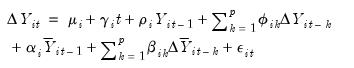
We may rewrite
Equation (42.102) in Augmented Dickey-Fuller form as
 | (42.103) |
where
, the

lagged differences are added to account for correlation in the

, and

represents factor augmentation.
It is important to highlight the fact that non-stationarity arises in this model only when the
autoregressive coefficient is equal to 0. Accordingly the null hypothesis for the unit root test is

for all
i,
against possibly heterogeneous alternatives,
such that
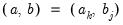
for

and

is a positive integer, where, without loss of generality, we reorder the cross-sections to facilitate partitioning by index
i.
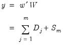
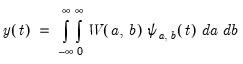
For

sufficiently large, Pesaran (2007) argues that
where
 | (42.104) |
are proxies for the common factor

. It follows that

and

may be used to filter out the effects of the unobserved common factor.
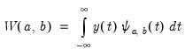
Using these proxies we obtain the cross-sectionally augmented ADF (CADF) equation:
 | (42.105) |
Let

denote the
t-statistic associated with the traditional ADF null hypothesis

for cross-section
i. Following Im, Pesaran, and Shin (2003), the panel unit root test of interest is a pooled version of individual CADF statistics, or the cross-sectionally augmented (CIPS) statistic:
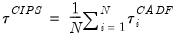 | (42.106) |
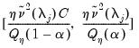
A truncated version of this test is proposed to counter the influence of extreme outcomes that may arise when

is sufficiently small, say

. Define the constants

and

obtained by simulation in Pesaran (2007), and use these values to define a truncated version of

,
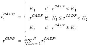 | (42.107) |
Neither CIPS nor truncated CIPS tests have standard limiting distributions. Critical values for popular scenarios have been derived via simulation and tabulated in Pesaran (2007).


 and
and  for
for  and
and  .
. of common factors, or use
  and
and  to determine
  , the number of factors to use (
“Determining the Number of Components”).
, the number of factors to use (
“Determining the Number of Components”). for
for  and
and  for
for 