Explosive Bubble Tests
Identification of bubbles in financial asset prices is an important topic in financial econometrics that has received considerable attention over the past decade (see Gürkaynak (2008) and Homm and Breitung (2012) for surveys of the literature).
EViews offers Phillips
et al.(2011, PWY) and Phillips
et al. (2015, PSY) tests for detection of bubbles. These tests are applications of ADF unit root tests (see
“The Augmented Dickey-Fuller (ADF) Test”) that are based on a model of asset prices of:
 | (42.17) |
Where

is the price of the asset,
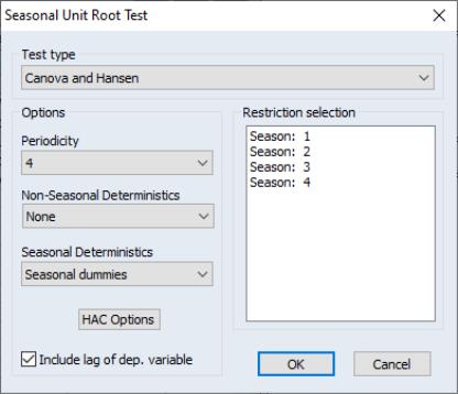
is the difference operator, and
is a given number of lags.
Under this model, a test for the presence of a bubble in the asset price is equivalent to testing for an explosion in the price,
i.e. an alternative hypothesis of

against a null hypothesis of a unit root,

, yielding a one-sided modification of the standard ADF test. Since explosive behavior is generally short-lived, tests for

will employ data observed over a short period, rather than the entire sample.
Given this framework, EViews computes three different bubble tests:
• The first method employs a series of rolling ADF (RADF) tests. In this framework, an initial ADF test is calculated over a short window of observations at the start of the data sample and the test statistic recorded. The procedure then rolls the window by one observation (both start date and end date are incremented by one) and an ADF test is computed and recorded. This process continue until the end of the data sample is reached. The maximum of the series of ADF statistics is the RADF test-statistic.
• PWY suggest an alternative approach which is to expand the window, rather than roll it. After estimating the initial small window, increment the end date of the sample by one at each iteration and compute the ADF. The maximum of these expanding statistics is termed the supremum ADF (SADF) test statistic.
• PSY generalize the procedure further by both rolling and expanding the window. The procedure begins by estimating the ADF for a small starting window, and then computing the expanding window SADF given that initial window. The window is then rolled by incrementing the start and end dates by one, and the SADF is computed given the new window. The process is repeated until we compute the SADF for the last of the rolling windows. The maximum of the SADF statistics computed given each of the rolling windows is the generalized supremum ADF (GSADF) statistic.
Note that the GSADF statistic may be thought of as a global statistic which, roughly speaking, evaluates all rolling and expanding possibilities. The method requires estimation of a very large number of ADF statistics when the sample size is large, and it may take a considerable amount of time to produce results.
The asymptotic distributions of the RADF, SADF, and GSADF test statistics are unknown, and critical values are obtained in EViews by bootstrap simulation.
Under the null hypothesis of a unit root, the ADF equation may be written as:
 | (42.18) |
We may estimate this equation for a given sample using least squares, and use the results to compute residuals,
, which we then demean.
For each bootstrap replication, we may resample from these residuals. Given resampled

, the

for the target sample may be generated using
Equation (42.18), using initial values of

taken from the original data, and the RADF, SADF or GSADF test statistic may be computed. This procedure is repeated many times to produce a distribution of test statistics from which critical or
p-values may be computed.
This view is available in non-panel workfiles.
To perform a bubble test in EViews, open the series and click on View/Time Series Diagnostics/Bubble Tests…
The Test type section controls which type of bubble test you would like to run. You may use the drop down menu to choose between: , , or .
As you choose the different methods, the label of the corresponding edit field will change to reflect the different role of the length setting:
• If is selected, the Window length edit field is used to specify the number of observations for each of the rolling tests.
• If is selected, the Initial window length edit field is used to specify the number of observations in the initial sample for of the expanding tests.
• If is selected, the Rolling window length edit field is used to specify the number of observations in each of the rolling windows upon which the expanding tests are based.
In the , you may specify the exogenous regressors to include in the ADF test equations. You may choose to include constant (Intercept), both a constant and a trend term (Trend and intercept), or neither (None).
You may use the
Lag length section of the dialog to control how many lagged difference terms
to include in the ADF test equation to account for autocorrelation. You may click on to let EViews automatically select
, or you may select and supply a positive integer value. If you choose automatic selection, you will be given options for specifying both the lag selection method (, , or ) and to be used in the selection procedure.
The Critical value section controls the calculation of critical values for output and display. You may set the level for the critical values in the edit field, and you may use the checkbox to customize the results graph.
The Bootstrap options section defines the options used for the bootstrap procedure used to produce the test p-values.
• The Replications edit field specifies the number of bootstrap simulations. The default of 9999 is set so that the bootstrap satisfies the integer conditions for optimal behavior at conventional test sizes (Davidson and MacKinnon, 2004, p. 165).
• The Random generator drop down menu lets you specify the type of random number generator used in the bootstrap simulations.
• You may enter a random number seed in the ed (optional) edit field. You may provide an integer value from 0 to 2,147,483,647, or you may the leave the edit field blank, in which case EViews will use the clock to obtain a seed.
See the description of
“Bootstrap Probabilities” for additional discussion.
To save series containing the ADF statistics for each period and the corresponding critical values, enter valid series names in the and edit fields, respectively.
Bubble Test Example
We consider the example data from Phillips, Shi, and Yu (2015), by downloading data from their webpage and generating the series SPRATIO:
wfopen(type=excel) https://img1.wsimg.com/blobby/go/e5e77e0b-59d1-44d9-ab25-4763ac982e53/downloads/ie_data.xls range=data colhead=5
pagecontract if date<>na
pagestruct @date(date)
series spratio = s_p_comp__p / dividend_d
spratio = spratio/@elem(spratio, "1871m1")*100
smpl @first 2010
We open SPRATIO and select View/Time Series Diagnostics/Bubble Tests…
and specify the test, with of 36, and a lag of 0. Click on to perform the test.
EViews will display a spool containing a test summary table and a graph of the ADF test statistics:
The summary table shows a test statistic value 3.4619 associated with the maximal value at 2008m08, an associated probability of 0.0007, so that the null hypothesis of no bubble is rejected.
The graph shows the path of the expanding ADF statistics used to construct the SADF statistic.


 is the price of the asset,
  is the difference operator, and
  is a given number of lags.
 against a null hypothesis of a unit root,
  , yielding a one-sided modification of the standard ADF test. Since explosive behavior is generally short-lived, tests for
  will employ data observed over a short period, rather than the entire sample.
 , which we then demean.
 , the
, the  for the target sample may be generated using
Equation (42.18), using initial values of
  taken from the original data, and the RADF, SADF or GSADF test statistic may be computed. This procedure is repeated many times to produce a distribution of test statistics from which critical or p-values may be computed.
 to include in the ADF test equation to account for autocorrelation. You may click on Automatic selection to let EViews automatically select
  , or you may select User specified and supply a positive integer value. If you choose automatic selection, you will be given options for specifying both the lag selection method (Akaike info criterion, Schwarz info criterion, or Hannan-Quinn info criterion) and Maximum lags to be used in the selection procedure.